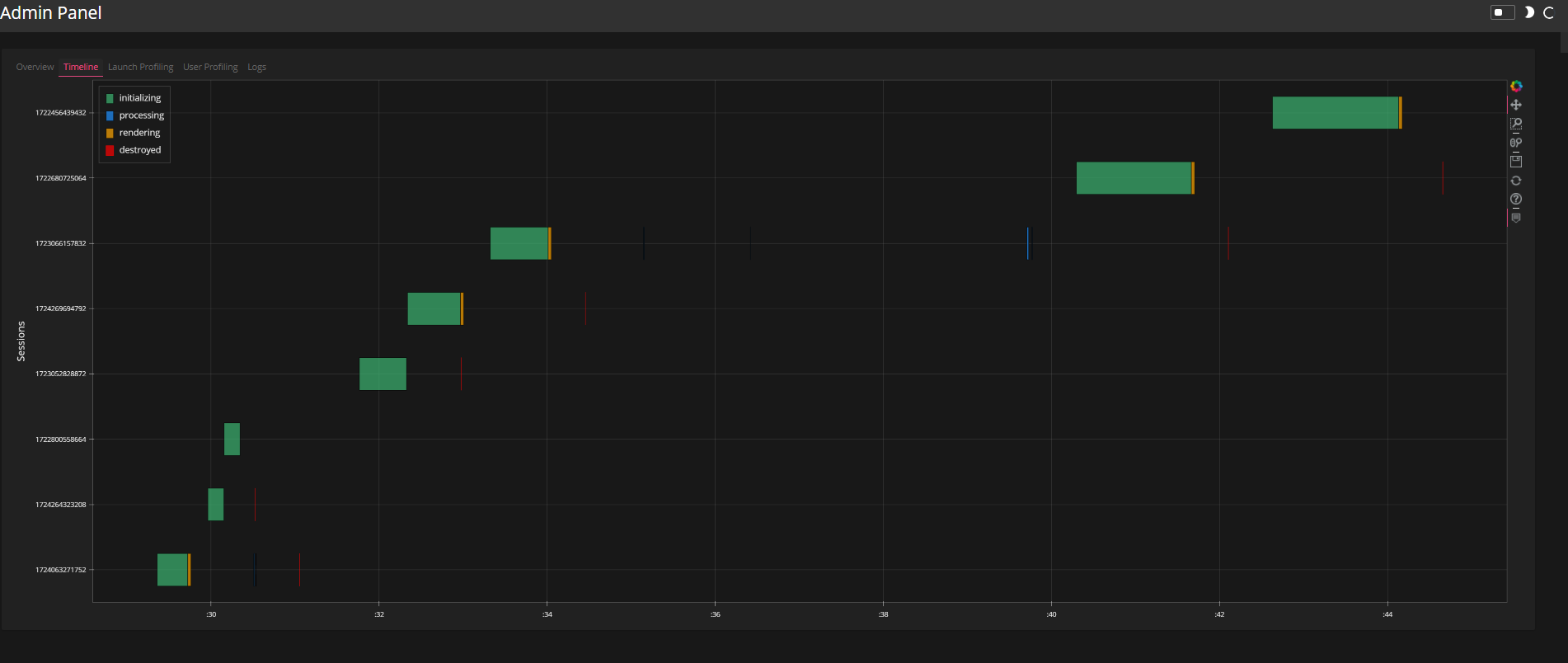
I was running your example (with panel 0.13.0a5.post19+ga2e4c848 and bokeh 2.4) and effectively it has some problem, but I could not see it. Sometimes the bokeh messages hass this problem of the bokeh referrers
and the app keeps increasing the memory each time 1 new session is launched.
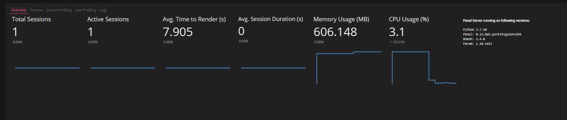
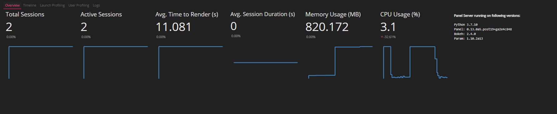
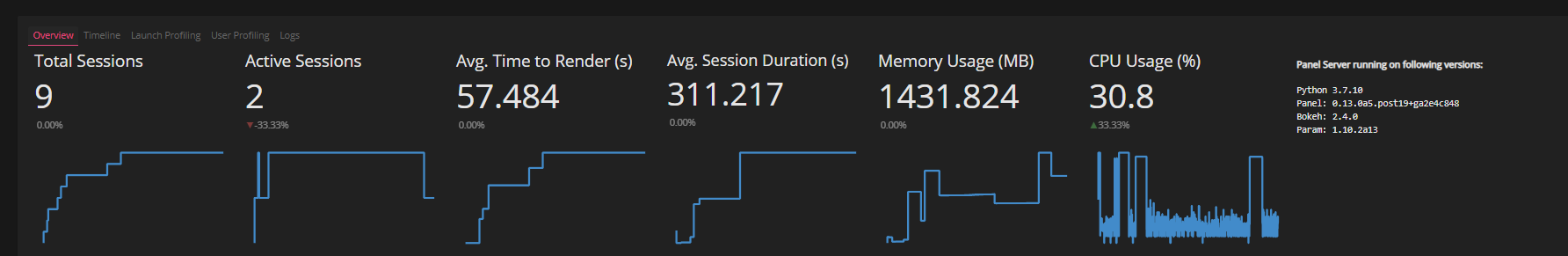
It begins with rendering time in 20 seconds and after 5 or 6 sessions it renders now in 110 seconds. Each time you run it, it increases 10 seconds. The memory begins in 600 Mb and it continues increasing till 1300 Mb now.
The app is really big and messy in order to debug, beyond my time capabilities. The only advice I have is related to avoid nested layout as much as you can. In some case you have inside a Tab something like pn.Column(pn.FlexBox(pn.indicators.Trend(w=200, h=200), which is completely unnecesary. In any case, the problem is not related to this, but with the memory leak. If you delete the column and the flexbox you reduce the rendering time by 1 or 2 seconds.
the first time
after one rendering
after several renderings
I copied the code below with several things deleted, but the improve is marginal as compared with the increase produced in each session. The data is the csv which was shared previously.
import numpy as np, pandas as pd
import panel as pn, time, datetime

import colorcet as cc
from colorcet.plotting import swatch

from bokeh.settings import settings
from bokeh.models import HoverTool
from bokeh.models.widgets.tables import DateFormatter,NumberFormatter
settings.resources = 'cdn'
settings.resources = 'inline'

import holoviews as hv
from holoviews import dim, opts
from holoviews.element import tiles
from holoviews.element.tiles import StamenTerrain

import hvplot.pandas
import datashader

pn.extension('tabulator',sizing_mode='stretch_width')

LSM_cmap = cc.CET_L4[::-1]

cus_compl = pd.read_csv('cust_compl.csv')
cus_compl['DATE'] = cus_compl['DATE'].astype('datetime64[ns]')
cus_compl['Month'] = cus_compl['DATE'].dt.month
cus_compl['Year'] = cus_compl['DATE'].dt.year
cus_compl['Month_Year'] = pd.to_datetime(cus_compl.Month.astype(str)+"-"+cus_compl.Year.astype(str))
cus_compl = cus_compl.reset_index()

cus_compl.drop_duplicates(inplace=True)


def create_trend(cus_compl):
    cus_compl_val = cus_compl.Month_Year.value_counts().rename_axis('Year_Month').reset_index(name='counts').sort_values(by='Year_Month')
    cus_compl_val['cum'] = cus_compl_val.counts.cumsum()
    cus_compl_val_daily = cus_compl[cus_compl.DATE> datetime.datetime.now() - pd.to_timedelta("30day")]['DATE'].dt.date.value_counts().rename_axis('Year_Month').reset_index(name='counts').sort_values(by='Year_Month')
    cus_compl_val_daily['cum'] = cus_compl_val_daily.counts.cumsum()

    data_daily = {'x': cus_compl_val_daily.index, 'y': cus_compl_val_daily.counts.values}
    data = {'x': cus_compl_val.index, 'y': cus_compl_val.counts.values}

    trend_monthly = pn.indicators.Trend(title='Nation Wide Trend', data=data, width=200, height=200)
    trend_daily = pn.indicators.Trend(title='Daily_Trend', data=data_daily, width=200, height=200)

    return trend_monthly,trend_daily


def create_trend_reg(cus_compl,reg):
    cus_compl_val = cus_compl[(cus_compl.RBU==reg)].Month_Year.value_counts().rename_axis('Year_Month').\
                    reset_index(name='counts').sort_values(by='Year_Month')
    cus_compl_val['cum'] = cus_compl_val.counts.cumsum()
    data = {'x': cus_compl_val.index, 'y': cus_compl_val.counts.values}
    trend_monthly = pn.indicators.Trend(title=F'{reg}', data=data, width=200, height=200)
    return trend_monthly

class groups:
    def complaint_grp_count(*arguments):
        '''
        time_v='30day'
        complaints='compl'
        relat=(Region,MBU,MSISDN,CITY,SiteCode)
        '''
        aList = list(arguments)
        if len(aList)>3:
            time_v=aList[-1]
        else:
            time_v="30day"

        aList = list(arguments)
        data = aList[0]
        groupby_wk = list(aList[1:-1])

        return data[data.DATE> datetime.datetime.now() - pd.to_timedelta(time_v)].groupby(groupby_wk)['MSISDN'].count().reset_index(name='counts').sort_values(by='counts')

    def site_grp_count():
        return cus_compl.groupby(['SiteCode','Month_Year',
            'compl','RBU','MBU','cityname','MSISDN','Longitude',
            'Latitute'])['MSISDN'].count().reset_index(name='counts').sort_values(by='counts')

    def msisdn_grp_count():
        return cus_compl.groupby(['MSISDN','Month_Year',
            'compl','RBU','MBU','cityname','SiteCode','Longitude',
            'Latitute'])['SiteCode'].count().reset_index(name='counts').sort_values(by='counts')

    def monthly_grp_count():
        return cus_compl.groupby(['Month_Year',
            'compl','RBU','MBU','cityname',
            'SiteCode'])['MSISDN'].count().reset_index(name='counts').sort_values(by='counts')


def rbu_heatmap():

    rbu_heatmap_comp = groups.monthly_grp_count().hvplot.heatmap(title='Complaints w.r.t Regions',x='Month_Year',
                        y='compl',groupby='RBU', C='counts', reduce_function=np.sum ,cmap=LSM_cmap,colorbar=True,
                        height=500,width=750).opts(toolbar=None )

    rbu_heatmap_mbu = groups.monthly_grp_count().hvplot.heatmap(title='Complaints w.r.t MBU',x='Month_Year', y='MBU',
                        groupby='RBU', C='counts', reduce_function=np.sum ,cmap=LSM_cmap,colorbar=True,height=500,
                        width=750).opts(toolbar=None )

    rbu_heatmap_city = groups.monthly_grp_count()[groups.monthly_grp_count().counts>20]\
        .hvplot.heatmap(title='Complaints w.r.t Cities',x='Month_Year', y='cityname',groupby='RBU',
        C='counts', reduce_function=np.sum ,cmap=LSM_cmap,colorbar=True,height=500,width=750).opts(toolbar=None )

    rbu_heatmap_comp = rbu_heatmap_comp.opts(tools=[HoverTool(tooltips=[('Complaint',"@compl"),('Count',"@counts"),
                       ('Month', '@{Month_Year}{%Y-%m}'),], formatters={'@{Month_Year}': 'datetime' })])
    rbu_heatmap_mbu = rbu_heatmap_mbu.opts(tools=[HoverTool(tooltips=[('MBU',"@MBU"),('Count',"@counts"),
                       ('Month', '@{Month_Year}{%Y-%m}'),],formatters={'@{Month_Year}': 'datetime'})])
    rbu_heatmap_city = rbu_heatmap_city.opts(tools=[HoverTool(tooltips=[('City',"@cityname"),('Count',"@counts"),
                          ('Month', '@{Month_Year}{%Y-%m}'),],formatters={'@{Month_Year}': 'datetime'})])
    rbu_heatmap_temp = (rbu_heatmap_comp+rbu_heatmap_mbu+rbu_heatmap_city).cols(2)
    rbu_heatmap_total = pn.panel(rbu_heatmap_temp,widgets={'RBU': pn.widgets.Select},widget_location='top_left')

    return rbu_heatmap_total


def nwd_trends():
    yearly_comp_gph = groups.complaint_grp_count(cus_compl,'Month_Year','compl',"1200day").hvplot.scatter(x='Month_Year',y='counts',by='compl',dynamic=True,shared_axes=False,use_index=False,legend='right')\
    .opts(toolbar=None,height=500,width=1000).opts(opts.Scatter(color=hv.Cycle('Category20'), line_color='k',size=dim('counts')/700,
                       show_grid=True, width=1000, height=1400), opts.NdOverlay(legend_position='left', show_frame=False)        )

    year_reg_grp = groups.complaint_grp_count(cus_compl,'Month_Year','compl','Region',"1200day")\
               .hvplot.line(x='Month_Year',y='counts',by='compl',groupby='Region',\
                    width=1550, height=600, dynamic=True,shared_axes=False).layout().cols(1).relabel('Complaints Trends')

    top_msisdn_comp_gph = groups.complaint_grp_count(cus_compl,'MSISDN','compl','30Days').sort_values(by='counts').nlargest(10,'counts').sort_values(by='counts')\
        .hvplot.barh(title='Top 10 Numbers', x='MSISDN',y='counts',by='compl',stacked=True,
        shared_axes=False).opts(toolbar=None,width=900, height=500)

    top_reg_comp_gph = groups.complaint_grp_count(cus_compl,'Region','compl','30Days').sort_values(by='counts')\
        .hvplot.barh(title='Region Wise',x='Region',y='counts',by='compl',stacked=True,
        shared_axes=False).opts(toolbar=None,width=900, height=500)

    top_city_comp_gph = groups.complaint_grp_count(cus_compl,'CITY','compl','30Days').sort_values(by='counts').nlargest(30,'counts').sort_values(by='counts')\
        .hvplot.barh(title='Top 30 Cities',x='CITY',y='counts',by='compl',stacked=True,
        shared_axes=False).opts(toolbar=None,width=900, height=500).sort(['compl','CITY'],reverse=True)

    top_mbu_comp_gph = groups.complaint_grp_count(cus_compl,'MBU','compl','30Days').sort_values(by='counts').nlargest(15,'counts').sort_values(by='counts')\
        .hvplot.barh(title='Top 15 MBU',x='MBU',y='counts',by='compl',stacked=True,
        shared_axes=False).opts(toolbar=None,width=900, height=500)

    top_site_comp_gph = groups.complaint_grp_count(cus_compl,'SiteCode','compl','30Days').sort_values(by='counts').nlargest(20,'counts').sort_values(by='counts')\
    .hvplot.barh(title='Top 20 Sites',x='SiteCode',y='counts',by='compl',stacked=True,shared_axes=False).opts(toolbar=None,width=900, height=500)

    comp_perc_gph = ((groups.complaint_grp_count(cus_compl,'compl','30Days').set_index('compl').plot.pie(y='counts',title="Complaints", legend=False, \
                       autopct='%1.1f%%', \
                       shadow=False,figsize=(10,10),ylabel='',\
                    startangle = 180)).get_figure())

    daily_trends = pn.Column(pn.Spacer(height=30),\
                        pn.Row(create_trend(cus_compl)[1],pn.pane.Matplotlib(comp_perc_gph,dpi=450)) ,\
                        pn.Spacer(height=30),\
                        pn.pane.Markdown("## Top Last 30 days Trends", sizing_mode="stretch_width"),\
           (top_reg_comp_gph+top_mbu_comp_gph+top_city_comp_gph+top_msisdn_comp_gph+top_site_comp_gph).cols(2),\
    sizing_mode='stretch_width')

    yearly_trends = pn.Column( pn.Spacer(height=30),create_trend(cus_compl)[0],pn.Spacer(height=30),
                        pn.Row(create_trend_reg(cus_compl,'South'),create_trend_reg(cus_compl,'North'),
                        create_trend_reg(cus_compl,'Central B'),create_trend_reg(cus_compl,'Central A')  ),
                        year_reg_grp.relabel('Yearly Complaints Analysis')                 )

    return pn.Row(pn.Tabs(('Yearly_Trends',yearly_trends),('Daily_Trends',daily_trends),tabs_location='above',dynamic=True))


def cust_mapping():
    cust_group_by_date=pd.DataFrame(groups.site_grp_count())
    x, y = datashader.utils.lnglat_to_meters(cust_group_by_date.Longitude, cust_group_by_date.Latitute)
    cust_group_by_work_projected = cust_group_by_date.join([pd.DataFrame({'easting': x}), pd.DataFrame({'northing': y})])

    RBU_select = pn.widgets.Select(name='RBUs', options=list(cust_group_by_work_projected.RBU.unique()))
    City_select =  pn.widgets.Select(name='CityLevel', options=list(sorted(cust_group_by_work_projected.cityname.unique())))
    Complaint_select = pn.widgets.MultiSelect(name='Complaints', options=list(sorted(cust_group_by_work_projected.compl.unique())))

    Month = pn.widgets.DateRangeSlider( name='Month',
        start=cust_group_by_work_projected.Month_Year.min(), end=cust_group_by_work_projected.Month_Year.max(),
        value=(cust_group_by_work_projected.Month_Year.min(), cust_group_by_work_projected.Month_Year.max()))

    hv.extension('bokeh')
    levels=[2,4,5]
    colors=['#0000FF','#FFFF00','#FF0000']

    wiki = tiles.StamenTerrain().redim(x='easting', y='northing')

    cust_group_by_work_hol=cust_group_by_work_projected.hvplot.points(x='easting', y='northing', c='counts',
        hover_cols=['SiteCode', 'Month_Year','RBU','MBU','cityname','compl'], s='counts',scale=10, cmap=colors,
        height=850, width=1550 , xaxis=None, yaxis=None,use_index=False, legend=False,colorbar=True,
        dynamic=True).opts(toolbar='above').opts(tools=[HoverTool(tooltips=[('SiteCode',"@SiteCode"),
            ('Complaint',"@compl"),('Count',"@counts"),('Month', '@{Month_Year}{%Y-%m}'),('MBU', '@{MBU}'),
            ('RBU',"@RBU"), ('City', "@cityname"), (' ',"==============="),],
             formatters={'@{Month_Year}': 'datetime'})])

    cust_group_by_work_hol=cust_group_by_work_hol.apply.opts(xticks=[1,3,5], clabel='Customer Complaints',clim=(1,10),color_levels=3,cmap='rainbow',
        colorbar_opts={  'major_label_overrides': { 0: 'none', 2: 'low',  5: 'high'    }       }        )

    cust_group_date_wise_b=wiki * (cust_group_by_work_hol.opts(toolbar='left')).apply.select(Month_Year=Month.param.value,
                cityname=City_select.param.value,compl=Complaint_select.param.value,watch=True)

    widgets = pn.WidgetBox(City_select,Complaint_select,Month,sizing_mode='fixed')
    date_format={'Month_Year': DateFormatter(), }
    filter_table=pn.widgets.Tabulator(cust_group_by_work_projected, pagination='remote', groupby=['Month_Year'],
        width=800,layout='fit_data_table', formatters=date_format, show_index=False, )

    filter_table.add_filter(City_select,'cityname')
    filter_table.add_filter(Complaint_select,'compl')
    filter_table.add_filter(Month,'Month_Year')

    return pn.Column(widgets,pn.Column(cust_group_date_wise_b.opts(width=1550),filter_table),sizing_mode='fixed')


def msidn_menu():
    MSISDN_select = pn.widgets.Select(name='MSISDN', options=list(sorted(groups.msisdn_grp_count().nlargest(30,'counts').sort_values(by='counts').MSISDN.unique())))
    date_format={  'Month_Year': DateFormatter(),   'MSISDN': NumberFormatter(format='0'),   }
    MSISDN_table=pn.widgets.Tabulator(groups.msisdn_grp_count().sort_values(by='counts'),pagination='remote', groupby=['MSISDN'],\
                                      width=800,layout='fit_data_table',formatters=date_format,show_index=False,)
    MSISDN_table.add_filter(MSISDN_select,'MSISDN')
    return pn.Column(MSISDN_select,MSISDN_table)


tab_dash=pn.Tabs(
         ('Nation Wide Trends',nwd_trends() ),
         ('Geo Mapping', cust_mapping()),
        ('Number Wise Complaints', msidn_menu()),
        ('Heat Maps',rbu_heatmap()),
       dynamic=True
    )

tmpl = pn.template.FastListTemplate(title='Customer Complaints')
tmpl.header_background='Red'
tmpl.header_color='Blue'
tmpl.title='Customer Complaints'

tmpl.main.append(tab_dash)

tmpl.servable('Customer Complaints')
I hope you find a solution.