Hi all!
I’m looking to optimize some code for plotting a very large set of neuronal spike times, and have found the hv.Spikes function to work very well. I want to try using hv.operation.decimate on top of the Spike object, but haven’t been able to yet.
Here is a simplified version that illustrates the issue:
data = np.random.randint(0, 100, 1000)
raster1 = hv.Spikes(data, kdims='Time')

x_r = (0, 100)
y_r = (0, 0.5)
decimate(raster1)
Which produces the error: WARNING:param.dynamic_operation: Callable raised "ValueError('not enough values to unpack (expected 2, got 1)')". Invoked as dynamic_operation(x_range=None, y_range=None)
Does anyone have an idea about how best to combine these two features, if possible? Thanks!
We should indeed improve decimate, but for now you can simply roll your own version like this:
data = np.random.randn(100000)
raster1 = hv.Spikes(data, kdims='Time')

x_range = hv.streams.RangeX(x_range=raster1.range(0))

def subsample(spikes, x_range, n=1000):
    sliced = spikes.select(Time=x_range)
    count = len(sliced)
    if count <= n:
        return sliced
    return sliced.iloc[np.random.randint(0, count, n)]

raster1.apply(subsample, streams=[x_range])
1 Like
This is very helpful, thank you!
One of the decimate functions that is really useful is that the plotting adjusts with zooming, so that if the resolution/downsampled points are gradually recovered with zooming in.
Would approach this by converting the raster plot into a HoloMap/DynamicMap, or is it simpler to add a while loop into the subsample function?
@barnold The function I supplied together with .apply and the RangeX stream should do exactly that too. When you zoom it’ll reveal more of spikes.
@philippjfr ah okay. in the toy code above, it’s difficult to tell how much the density changes. I implemented another toy version using your snippet and the NdOverlay objects to get closer to a final data version and found that the spike reveal feature isn’t present there.
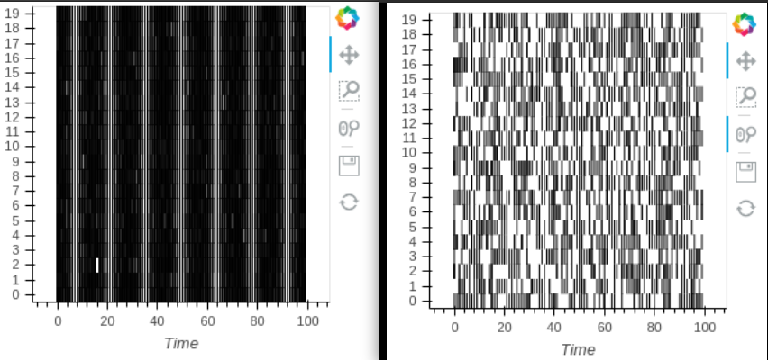
So with a slightly more complicated initial raster:
raster = hv.NdOverlay({i: hv.Spikes(np.random.randint(0, 100, 1000), kdims='Time').opts(position=0.1*i)
                   for i in range(20)}).opts(yticks=[((i+1)*0.1-0.05, i) for i in range(20)]).opts(
    opts.Spikes(spike_length=0.1),
    opts.NdOverlay(show_legend=False))
raster
and an adjusted version of your examples:
def raster_subsample(raster, x_range, n=100):
    new_spikes_objects = []
    for spikes in raster:
        sliced = spikes.select(Time=x_range)
        count = len(sliced)
        if count <= n:
            new_spikes_objects.append(sliced)
            continue
        new_spikes_objects.append(sliced.iloc[np.random.randint(0, count, n)])

    new_overlay = hv.NdOverlay({j: new_spikes_objects[j] for j in     range(len(new_spikes_objects))}).opts(yticks=[((j+1)*0.1-0.05, j) for j in range(20)]).opts(
        opts.Spikes(spike_length=0.1),
        opts.NdOverlay(show_legend=False))

    return new_overlay

x_span = (0, 100)
x_range = hv.streams.RangeX(x_range=x_span)

raster.apply(raster_subsample, streams=[x_range])
I manually redefine the x range here, otherwise only the index of each hv.Spike object is pulled.
In this case, the total number of spikes that are plotted remains constant with zooming (right raster, versus original on the left). Is there a more “holoviews” way of defining the x-range that might fix this?
Many thanks for your time and input!