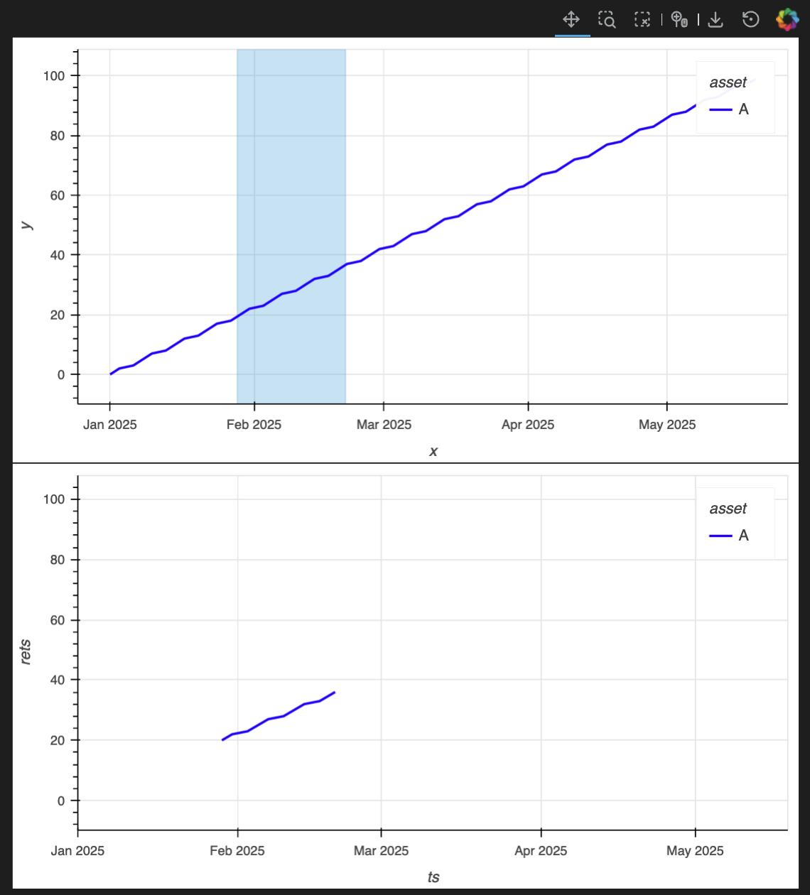
I have created a layout with two plots. The top plot show the full data and allows selection of a date range. The bottom plot is supposed to show just the data over the selected region. I would like the bottom plot’s x and y- limits to rescale to the data being shown. I can’t get this to work despite playing with shared_axes=False and framewise=True. Any help would be greatly appreciated!
Thanks
def plot_simple(
    returns: pd.DataFrame,
    *,
    figure_kwargs: dict | None = None,
) -> hv.core.layout.Layout:
    """Build an interactive HoloViews/Panel viewer of return indices with an
    overview-driven x-range selector.

    Parameters
    ----------
    returns : pandas.DataFrame
        Time-indexed periodic returns. The row index must be a single-level
        time index; its name is optional. Columns must be a simple Index (not
        MultiIndex). Return indices are computed via
        com.cat.strategies.utils.backtest.return_indices.
    facets : Mapping[Hashable, pandas.DataFrame] | None, optional
        Optional mapping of label -> DataFrame. Each DataFrame is reindexed to
        the main index and the main columns in returns; missing labels become
        NaN. The mapping key becomes the y-axis label of the facet panel.
        Facet DataFrames must have single-level columns.
    geometric : bool, keyword-only
        If True, compute a geometric cumprod index anchored at 1; if False,
        compute an arithmetic cumulative sum index. The overview and main
        panels use a logarithmic y-axis only when True; facet panels remain
        linear.
    facet_height_ratio : float, keyword-only
        Controls relative heights via GridSpec row allocation: the main panel
        spans int(1/facet_height_ratio) rows; each facet occupies one row. Must
        be > 0 (e.g., 0.33 makes the main ~3× a facet).
    hide_facet_legends : bool, keyword-only
        If True, hides legends on facet panels. The main panel legend is shown
        at the top-left.
    figure_kwargs : dict | None, keyword-only
        Extra keyword arguments forwarded to hv.opts.Curve for all panels.
        If None, sensible defaults are applied and used. When provided, the
        mapping is shallow-merged over defaults; user keys override defaults.
        Defaults are: responsive=True, show_grid=True, min_height=100,
        min_width=200, autorange='y', yformatter=NumeralTickFormatter(
        format='0.0%').
        By default, uses a percent tick formatter for y values.
    summary_fn : Callable[[pandas.DataFrame], Styler] | None, optional
        Function that returns a pandas Styler for a summary table computed over
        the selected window. By default, a per-column summary based on
        com.cat.strategies.utils.backtest.summary is computed and styled via
        returns.apply(summary, axis='index').style. The Styler is rendered in a
        Panel HTML pane and recomputed whenever the selection changes. Pass
        None to disable the summary.
    summary_table_opts : dict | None, keyword-only
        Panel HTML pane keyword arguments (e.g., styles, sizing_mode, margin).

    Returns
    -------
    pn.Row
        A Panel Row (sizing_mode='stretch_both') with one or two children:
        - A GridSpec containing:
          - Top row: an overview plot of the full-period return index with an
            interactive horizontal box-select (x-range) tool. The overview
            shows the x-axis at the top, hides the y-axis, and activates
            xbox_select with the toolbar hidden. A translucent band reflects
            the selection.
          - Below: a main plot that recomputes return indices for the selected
            window (anchored at the window start) and optional facet plots
            sliced and aligned to the same window.
        - When summary_fn is provided, an HTML summary pane rendering the
          Styler for the selected window.

    Raises
    ------
    AssertionError
        - If returns does not have a single-level row index.
        - If returns has MultiIndex columns.
        - If facet_height_ratio is not > 0.
        - If any facet DataFrame has MultiIndex columns.
        - If summary_fn is provided but is not callable.

    Notes
    -----
    - Selection normalization: selection bounds are validated, ordered, clipped
      to the data range, and robustly parsed (timestamps or epoch ms). If the
      selected window is empty, the full period is used.
    - Color mapping is deterministic by column label and is stable across all
      panels.
    - The overview’s axes are not shared with other panels. Main and facet
      panels are independent plots that update to the selected date range.
    - Panning is not available; use the overview’s box-select to choose a time
      window.
    - Selection summary: When summary_fn is provided, a tabular summary of the
      selected window is displayed alongside the plots and recomputed on each
      selection change.
    - See also: com.cat.strategies.utils.backtest.return_indices.
    """
    assert returns.index.nlevels == 1, (
        f"returns must have a single-level time index; got "
        f"{returns.index.nlevels} levels with names "
        f"{returns.index.names}"
    )
    assert returns.columns.nlevels == 1, (
        "returns must have a single-level columns Index "
        "(MultiIndex not supported)"
    )
    default_fig_kwargs = dict(
        responsive=True,
        show_grid=True,
        min_height=80,
        min_width=160,
        # yformatter=NumeralTickFormatter(format='0.0%'),
    )
    figure_kwargs = {**default_fig_kwargs, **(figure_kwargs or {})}

    # Precompute stable metadata from the full dataset.
    full_indices = returns.cumsum()
    time_name = full_indices.index.name or "time"

    overlay_dim = returns.columns.name or "column"

    # Deterministic color mapping by column label (stable across panels).
    categories = list(returns.columns.unique())

    base_palette = (
        Category10[10]
        + Category20[20]
        + Category20b[20]
        + Category20c[20]
    )
    colors = [
        base_palette[i % len(base_palette)] for i in range(len(categories))
    ]
    color_map = dict(zip(categories, colors))
    color_spec = hv.dim(overlay_dim).categorize(
        color_map, default="#9e9e9e"
    )

    # Helper: normalize selection bounds to valid [xmin, xmax] Timestamps.
    def normalize_bounds(boundsx, xmin, xmax):
        def to_ts(x):
            if x is None:
                return None
            if isinstance(x, pd.Timestamp):
                return x
            # Attempt robust conversion; treat numeric as epoch milliseconds.
            try:
                if isinstance(x, (int, float)):
                    return pd.to_datetime(x, unit="ms")
                return pd.to_datetime(x)
            except Exception:
                return None

        if boundsx is None or not isinstance(boundsx, (tuple, list)) \
                or len(boundsx) != 2:
            start, end = xmin, xmax
        else:
            start, end = to_ts(boundsx[0]), to_ts(boundsx[1])
            if start is None or end is None:
                start, end = xmin, xmax

        if start > end:
            start, end = end, start
        if start < xmin:
            start = xmin
        if end > xmax:
            end = xmax
        return start, end

    # Helper: build an overlay from a wide DataFrame of indices.
    def build_overlay_from_indices(
        idx_df: pd.DataFrame,
        ylabel: str,
        logy: bool,
        show_legend: bool,
        xaxis: str | None,
        extra_curve_opts: dict | None = None,
    ):
        stacked = idx_df.stack(future_stack=True)
        stacked.index.set_names([time_name, overlay_dim], inplace=True)
        stacked.name = ylabel

        ds_local = hv.Dataset(stacked.reset_index(), vdims=ylabel)
        overlay = ds_local.to(hv.Curve, kdims=time_name).overlay(overlay_dim)
        curve_opts = dict(
            ylabel=ylabel,
            logy=logy,
            tools=["hover"],
            color=color_spec,
            xaxis=xaxis,
            show_legend=show_legend,
            **figure_kwargs,
        )
        if extra_curve_opts:
            curve_opts.update(extra_curve_opts)
        overlay = overlay.options(
            hv.opts.Curve(**curve_opts),
            hv.opts.NdOverlay(legend_position="top_left"),
        )
        return overlay

    # Build the overview (full period) with range selection.
    xmin, xmax = full_indices.index.min(), full_indices.index.max()
    overview = build_overlay_from_indices(
        full_indices,
        ylabel="Return Index",
        logy=False,
        show_legend=False,
        xaxis="top",
        extra_curve_opts=dict(
            tools=["hover", "xbox_select"],
            yaxis=None, xlabel="", toolbar=None,
            active_tools=["xbox_select"]
        ),
    )
    overview.group = 'Overview'
    overview.label = 'Plot'

    sel = hv.streams.BoundsX(source=overview, boundsx=(xmin, xmax))

    sel_overlay = hv.DynamicMap(
        lambda boundsx: hv.VSpan(
            *normalize_bounds(boundsx, xmin, xmax)
        ).opts(
            color="gray",
            line_alpha=0,
            fill_alpha=0.15,
            show_legend=False,
        ),
        streams=[sel],
        group='Overview', label='Selection'
    ).options(framewise=True)
    overview_with_sel = (overview * sel_overlay)

    # Dynamic main plot: recompute indices on selection.
    def build_main(boundsx):
        start, end = normalize_bounds(boundsx, xmin, xmax)
        window_rets = returns.loc[start:end]
        if window_rets.empty:
            window_rets = returns
            start, end = xmin, xmax

        print(f"start: {start}, end: {end}")
        overlay = build_overlay_from_indices(
            window_rets.cumsum(),
            logy=False,
            ylabel="Return Index",
            show_legend=True,
            xaxis="bottom",
            extra_curve_opts=dict(
                active_tools=[],
                axiswise=True,
                xlim=(start, end)
            ),
        )
        return overlay

    main_panel = hv.DynamicMap(build_main, streams=[sel]).options(
        framewise=True
    )

    return (overview_with_sel + main_panel).cols(1).options(
        hv.opts.Layout(shared_axes=False)
    )
Call it using something like this:
import pandas as pd
import numpy as np

plot_simple(
    pd.DataFrame(
        np.random.randn(len(pd.date_range('2025-01-01', '2025-10-15', freq='B')), 5),
        columns=[f"Asset_{i+1}" for i in range(5)],
        index=pd.date_range('2025-01-01', '2025-10-15', freq='B')
    ),
    figure_kwargs=dict(height=300)
)