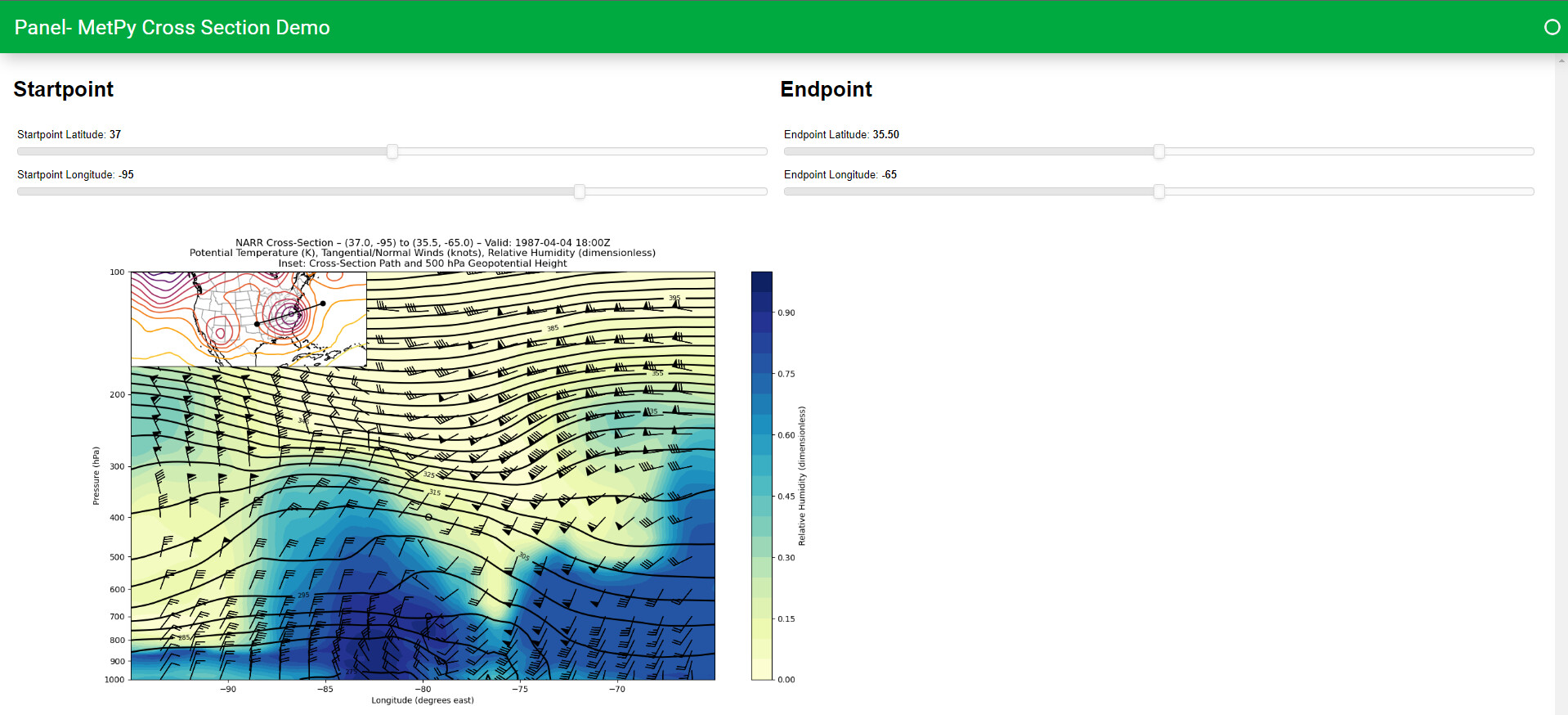
I am looking to create a replica of this Bokeh demo using normal NetCDF data and the MetPy Cross Section Analysis and I am not really sure how to even start or attempt this. I am looking for an explanation on how to replicate the Bokeh click to create path on which we cut the dataset on and then if possible how to hook the coordinates to a function that returns the resulting MetPy diagram. I have made a simple slider enabled demo that looks like
obtained using the following code :
import cartopy.crs as ccrs
import cartopy.feature as cfeature
import matplotlib.pyplot as plt
import numpy as np
import xarray as xr
import panel as pn
import metpy.calc as mpcalc
from metpy.cbook import get_test_data
from metpy.interpolate import cross_section

data = xr.open_dataset(get_test_data('narr_example.nc', False))
data = data.metpy.parse_cf().squeeze()

pn.extension(sizing_mode = 'stretch_width', template="material")
pn.state.template.param.update(site="Panel", title="MetPy Cross Section Demo")

startlat = pn.widgets.FloatSlider(name='Startpoint Latitude', start=17., end=57., step=10., value=37., value_throttled=10.0)
startlon = pn.widgets.FloatSlider(name='Startpoint Longitude', start=-125., end=-85., step=10., value=-105., value_throttled=10.0)

endlat = pn.widgets.FloatSlider(name='Endpoint Latitude', start=15.5, end=55.5, step=10., value=35.5, value_throttled=10.0)
endlon = pn.widgets.FloatSlider(name='Endpoint Longitude', start=-85., end=-45., step=10., value=-65.0, value_throttled=10.0)


def getFig(slat: int, slon: int, elat: int, elon: int):
    start = (slat,slon)
    end = (elat,elon)
    cross = cross_section(data, start, end).set_coords(('lat', 'lon'))
    cross['Potential_temperature'] = mpcalc.potential_temperature(
        cross['isobaric'],
        cross['Temperature']
    )
    cross['Relative_humidity'] = mpcalc.relative_humidity_from_specific_humidity(
        cross['isobaric'],
        cross['Temperature'],
        cross['Specific_humidity']
    )
    cross['u_wind'] = cross['u_wind'].metpy.convert_units('knots')
    cross['v_wind'] = cross['v_wind'].metpy.convert_units('knots')
    cross['t_wind'], cross['n_wind'] = mpcalc.cross_section_components(
        cross['u_wind'],
        cross['v_wind']
    )

    # Define the figure object and primary axes
    fig = plt.figure(figsize=(16., 9.))
    ax = plt.axes()

    # Plot RH using contourf
    rh_contour = ax.contourf(cross['lon'], cross['isobaric'], cross['Relative_humidity'],
                             levels=np.arange(0, 1.05, .05), cmap='YlGnBu')
    rh_colorbar = fig.colorbar(rh_contour)

    # Plot potential temperature using contour, with some custom labeling
    theta_contour = ax.contour(cross['lon'], cross['isobaric'], cross['Potential_temperature'],
                               levels=np.arange(250, 450, 5), colors='k', linewidths=2)
    theta_contour.clabel(theta_contour.levels[1::2], fontsize=8, colors='k', inline=1,
                         inline_spacing=8, fmt='%i', rightside_up=True, use_clabeltext=True)

    # Plot winds using the axes interface directly, with some custom indexing to make the barbs
    # less crowded
    wind_slc_vert = list(range(0, 19, 2)) + list(range(19, 29))
    wind_slc_horz = slice(5, 100, 5)
    ax.barbs(cross['lon'][wind_slc_horz], cross['isobaric'][wind_slc_vert],
             cross['t_wind'][wind_slc_vert, wind_slc_horz],
             cross['n_wind'][wind_slc_vert, wind_slc_horz], color='k')

    # Adjust the y-axis to be logarithmic
    ax.set_yscale('symlog')
    ax.set_yticklabels(np.arange(1000, 50, -100))
    ax.set_ylim(cross['isobaric'].max(), cross['isobaric'].min())
    ax.set_yticks(np.arange(1000, 50, -100))

    # Define the CRS and inset axes
    data_crs = data['Geopotential_height'].metpy.cartopy_crs
    ax_inset = fig.add_axes([0.125, 0.665, 0.25, 0.25], projection=data_crs)

    # Plot geopotential height at 500 hPa using xarray's contour wrapper
    ax_inset.contour(data['x'], data['y'], data['Geopotential_height'].sel(isobaric=500.),
                     levels=np.arange(5100, 6000, 60), cmap='inferno')

    # Plot the path of the cross section
    endpoints = data_crs.transform_points(ccrs.Geodetic(),
                                          *np.vstack([start, end]).transpose()[::-1])
    ax_inset.scatter(endpoints[:, 0], endpoints[:, 1], c='k', zorder=2)
    ax_inset.plot(cross['x'], cross['y'], c='k', zorder=2)

    # Add geographic features
    ax_inset.coastlines()
    ax_inset.add_feature(cfeature.STATES.with_scale('50m'), edgecolor='k', alpha=0.2, zorder=0)

    # Set the titles and axes labels
    ax_inset.set_title('')
    ax.set_title(f'NARR Cross-Section \u2013 {start} to {end} \u2013 '
                 f'Valid: {cross["time"].dt.strftime("%Y-%m-%d %H:%MZ").item()}\n'
                 'Potential Temperature (K), Tangential/Normal Winds (knots), Relative Humidity '
                 '(dimensionless)\nInset: Cross-Section Path and 500 hPa Geopotential Height')
    ax.set_ylabel('Pressure (hPa)')
    ax.set_xlabel('Longitude (degrees east)')
    rh_colorbar.set_label('Relative Humidity (dimensionless)')

    return fig

finalFigure = pn.bind(getFig, slat=startlat, slon=startlon, elat=endlat, elon=endlon)

latloncontrols = pn.Row(
    pn.Column(
        pn.pane.Markdown("""# Startpoint"""),
        startlat,
        startlon
    ),
    pn.Column(
        pn.pane.Markdown("""# Endpoint"""),
        endlat,
        endlon
    )
)
latloncontrols.servable(target='main')
pn.panel(finalFigure).servable(target='main')