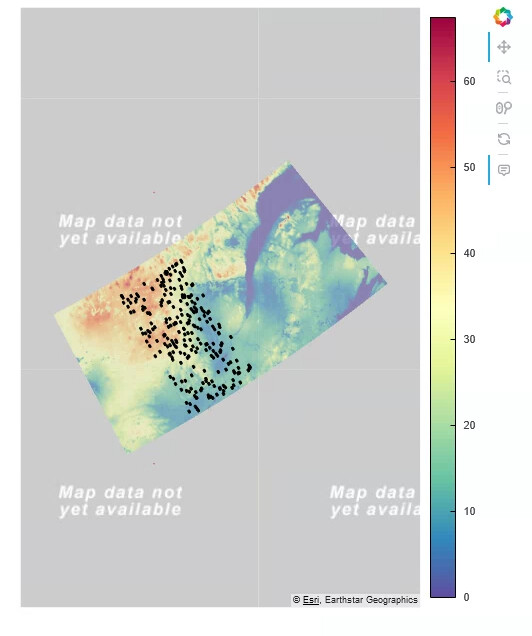
I’m currently following an online tutorial on how to perform an interactive visualization of an xarray dataset, but i’m also integrating geodataframe boundaries into the visualization with geoviews. While I am able to load the dataset and add the geopandas fields, I’m running into a few issues: I lose properties such as the Esri imagery and the grid no longer appears rotated. I attached an image at the end of the post that shows a print screen of the final plot.
I am using PyCharm Professional Edition 2023.3.2 with the Jupyter Notebook extension.
Can anybody tell me what’s going on? Cheers!
# read dataset
ds = xr.open_mfdataset(["\...\2021011506_000.nc"])

# Subset over all regions (need the geojson for this)
fields_geojson = gpd.GeoDataFrame.from_file("\...\rectangular_polygons.geojson")
fields_geojson = fields_geojson.set_crs('epsg:4326')

# Create subset based on the boundary limits of the fields
total_bounds = fields_geojson.geometry.total_bounds
min_lon, min_lat, max_lon, max_lat = total_bounds

# Create the crs based on the xarray dataset's metadata
rotp = ccrs.RotatedPole(
    pole_longitude=tmp_bbox.rotated_pole.grid_north_pole_longitude,
    pole_latitude=tmp_bbox.rotated_pole.grid_north_pole_latitude,
)

# Plotting the geodataframe with geoviews
gv_polygons = gv.Polygons(fields_geojson, vdims=['noChamp']).opts(
    alpha=1, line_color='black', projection=rotp, fill_color=None
)

# Create the map plot from the xarray dataset
map1 = ds.CaLDAS_A_SD_Avg.hvplot.quadmesh(
    x="rlon",
    y="rlat",
    cmap='Spectral_r',
    geo=True,
    crs=rotp,
    tiles='EsriImagery',
    frame_width=400,
    frame_height=600,
    dynamic=False,
    alpha=0.8
)

# combine dataset and geopandas
combined_plot = map1 * gv_polygons
print(ds)
<xarray.Dataset>
Dimensions:          (rlat: 460, rlon: 522, time: 1)
Coordinates:
    lat              (rlat, rlon) float32 dask.array<chunksize=(460, 522), meta=np.ndarray>
    lon              (rlat, rlon) float32 dask.array<chunksize=(460, 522), meta=np.ndarray>
  * time             (time) datetime64[ns] 2021-01-15T06:00:00
  * rlat             (rlat) float32 -2.965 -2.943 -2.92 ... 7.318 7.34 7.363
  * rlon             (rlon) float32 21.47 21.49 21.52 ... 33.15 33.17 33.19
Data variables:
    CaLDAS_P_I2_SFC  (time, rlat, rlon) float32 dask.array<chunksize=(1, 460, 522), meta=np.ndarray>
    CaLDAS_P_DN_SFC  (time, rlat, rlon) float32 dask.array<chunksize=(1, 460, 522), meta=np.ndarray>
    CaLDAS_A_SD_Veg  (time, rlat, rlon) float32 dask.array<chunksize=(1, 460, 522), meta=np.ndarray>
    CaLDAS_A_SD_Avg  (time, rlat, rlon) float32 dask.array<chunksize=(1, 460, 522), meta=np.ndarray>
    rotated_pole     float32 ...
Attributes:
    product:      CaLDAS
    Conventions:  CF-1.6
    Remarks:      Variable names are following the convention <Product>_<Type...
    License:      These data are provided by the Canadian Surface Prediction ...
print(fields_geojson)
                                              geometry
0    POLYGON ((-75.23822 45.81036, -75.13822 45.810...
1    POLYGON ((-73.33674 46.69549, -73.23674 46.695...
2    POLYGON ((-73.55984 48.37041, -73.45984 48.370...
3    POLYGON ((-75.46064 46.19510, -75.36064 46.195...
4    POLYGON ((-75.64253 47.48844, -75.54252 47.488...
pn.serve(combined_plot)