Hey everyone,
I just started to get into Holoviews and had already some good fun with experimenting with some ICON data.
I’ve got the current task now to make an interactive plot of the date where it’s possible to see the change in time or height.
So far I was able to either make a static plot (no variation in height or time) or make an interactive plot, but there I wasn’t able to get the the TriMesh and the projection working. Has anyone an Idea how to solve that issue? Or is there a way to have a DynamicPlot in a Dynamicplot?
import cartopy.crs as ccrs
import cartopy.feature as cf
import datashader as ds
import geoviews as gv
import geoviews.feature as gf
import holoviews as hv
import numpy as np
import pandas as pd
import xarray as xr
from holoviews import opts
from holoviews.operation.datashader import datashade, rasterize, regrid
from scipy.spatial import Delaunay
from bokeh.io import output_notebook, show
from bokeh.plotting import figure
import matplotlib.pyplot as plt

datashade.precompute = True

hv.extension("bokeh")
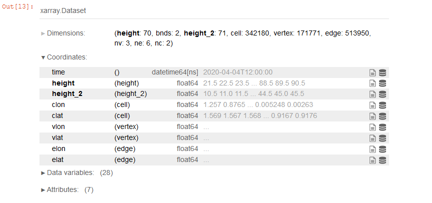
def merge(data_file, grid_data, path = './'):
    """
    Merging the data with the grid file and returs the merged x-array
    args: data x-array, grid x-array
    returns: merged x-array
    """

    data = xr.open_dataset(path+data_file)
    grid_data = xr.open_dataset(path+grid_data)

    return xr.merge([data.rename({'ncells': 'cell'}), grid_data])


def triangulate(vertices, x="Longitude", y="Latitude"):
    """
    Generate a triangular mesh for the given x,y,z vertices, using Delaunay triangulation.
    For large n, typically results in about double the number of triangles as vertices.
    """
    triang = Delaunay(vertices[[x, y]].values)
    return pd.DataFrame(triang.simplices, columns=['v0', 'v1', 'v2'])


def calc(pressure):
    pts = np.stack((x, y, pressure)).T
    verts = pd.DataFrame(pts, columns=['Longitude', 'Latitude', 'pres'])
    tris = triangulate(verts)
    return verts, tris
data_file = "20200404_12_ana.nc"
grid_data = "icon_grid.nc"

data = merge(data_file, grid_data)
data = data.isel(time=0)

x = ((np.rad2deg(data.clon) - 180) % 360) - 180
y = np.rad2deg(data.clat)
data
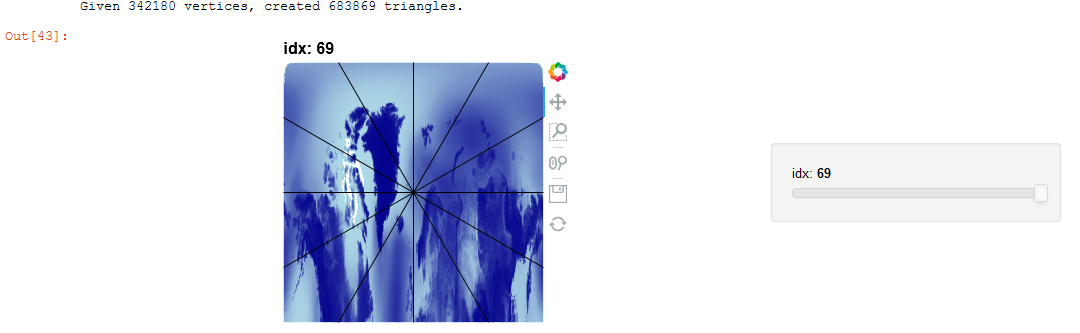
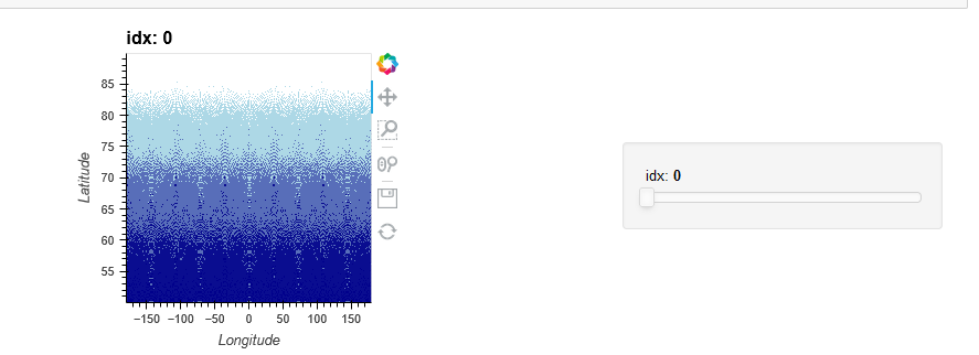
def points(idx, data = data):
    verts, tris = calc(data.pres[idx])
    return rasterize(hv.Points(verts, vdims='pres'), dynamic = False)
    #return hv.TriMesh(rasterize(hv.Points(verts, vdims='pres'), dynamic = False)) <- not working
img = datashade(hv.DynamicMap(points, kdims=['idx']))
img.redim.range(idx=(0,69))
following followed by source
graticules = cf.NaturalEarthFeature(
category='physical',
name='graticules_30',
scale='50m')
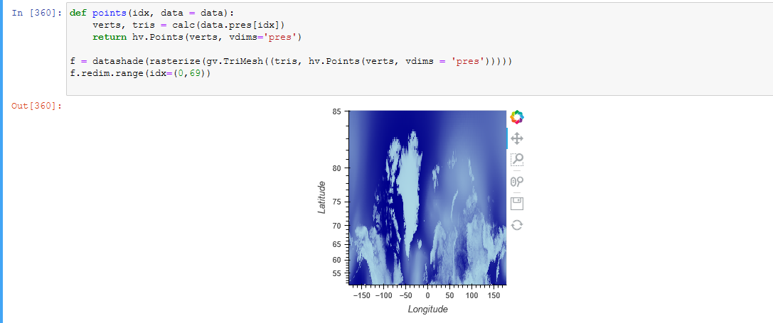
verts, tris = calc(data.pres[-1])
trimesh = rasterize(
gv.TriMesh(
(tris, hv.Points(verts, vdims='pres')),
label="pressure in Pa",
crs=ccrs.PlateCarree(),
),
aggregator=ds.mean('pres'),
)
(trimesh).opts(
colorbar=True, alpha = 0.99, cmap = 'cividis',width=500, height=500, projection=ccrs.NorthPolarStereo()
) * gf.coastline * gf.borders * gv.Feature(graticules, group='Lines')

I also managed to do this, but got stuck there: (animation still doesn’t work)