Hi,
I am little new to bokeh dynamic property part,
I have made simple program related to my plot sample plot where i can generating data in script itself and plotted .
As previous plot is acting dynamic in jupyter when using bokeh server but while bokeh plot embedding into flask dynamic nature of plot vanish . 
I am struggling with callback function to write,I don’t know how to change and where as i am using holomap concept,
Kindly help me out.
MY minimal example :
Test.py
from flask import Flask, render_template
from werkzeug.wrappers import Request, Response
from bokeh.embed import file_html
from flask import Flask,Markup
app = Flask( **name** )
@app.route('/plot')
def plot():
    import numpy as np
    import pandas as pd
    import geoviews as gv
    import holoviews as hv
    import panel as pn
    from holoviews.operation.datashader import rasterize
    hv.extension("bokeh")
    from bokeh.models.callbacks import CustomJS
    # Some points defining a triangulation over (roughly) Britain.
    xy = np.asarray([
        [-0.101, 0.872], [-0.080, 0.883], [-0.069, 0.888], [-0.054, 0.890],
        [-0.045, 0.897], [-0.057, 0.895], [-0.073, 0.900], [-0.087, 0.898],
        [-0.090, 0.904], [-0.069, 0.907], [-0.069, 0.921], [-0.080, 0.919],
        [-0.073, 0.928], [-0.052, 0.930], [-0.048, 0.942], [-0.062, 0.949],
        [-0.054, 0.958], [-0.069, 0.954], [-0.087, 0.952], [-0.087, 0.959],
        [-0.080, 0.966], [-0.085, 0.973], [-0.087, 0.965], [-0.097, 0.965],
        [-0.097, 0.975], [-0.092, 0.984], [-0.101, 0.980], [-0.108, 0.980],
        [-0.104, 0.987], [-0.102, 0.993], [-0.115, 1.001], [-0.099, 0.996],
        [-0.101, 1.007], [-0.090, 1.010], [-0.087, 1.021], [-0.069, 1.021],
        [-0.052, 1.022], [-0.052, 1.017], [-0.069, 1.010], [-0.064, 1.005],
        [-0.048, 1.005], [-0.031, 1.005], [-0.031, 0.996], [-0.040, 0.987],
        [-0.045, 0.980], [-0.052, 0.975], [-0.040, 0.973], [-0.026, 0.968],
        [-0.020, 0.954], [-0.006, 0.947], [0.003, 0.935], [0.006, 0.926],
        [0.005, 0.921], [0.022, 0.923], [0.033, 0.912], [0.029, 0.905],
        [0.017, 0.900], [0.012, 0.895], [0.027, 0.893], [0.019, 0.886],
        [0.001, 0.883], [-0.012, 0.884], [-0.029, 0.883], [-0.038, 0.879],
        [-0.057, 0.881], [-0.062, 0.876], [-0.078, 0.876], [-0.087, 0.872],
        [-0.030, 0.907], [-0.007, 0.905], [-0.057, 0.916], [-0.025, 0.933],
        [-0.077, 0.990], [-0.059, 0.993]])
    # Make lats + lons
    x = abs(xy[:, 0] * 180 / 3.14159)
    y = xy[:, 1] * 180 / 3.14159

    # A selected triangulation of the points.
    triangles = np.asarray([
        [67, 66, 1], [65, 2, 66], [1, 66, 2], [64, 2, 65], [63, 3, 64],
        [60, 59, 57], [2, 64, 3], [3, 63, 4], [0, 67, 1], [62, 4, 63],
        [57, 59, 56], [59, 58, 56], [61, 60, 69], [57, 69, 60], [4, 62, 68],
        [6, 5, 9], [61, 68, 62], [69, 68, 61], [9, 5, 70], [6, 8, 7],
        [4, 70, 5], [8, 6, 9], [56, 69, 57], [69, 56, 52], [70, 10, 9],
        [54, 53, 55], [56, 55, 53], [68, 70, 4], [52, 56, 53], [11, 10, 12],
        [69, 71, 68], [68, 13, 70], [10, 70, 13], [51, 50, 52], [13, 68, 71],
        [52, 71, 69], [12, 10, 13], [71, 52, 50], [71, 14, 13], [50, 49, 71],
        [49, 48, 71], [14, 16, 15], [14, 71, 48], [17, 19, 18], [17, 20, 19],
        [48, 16, 14], [48, 47, 16], [47, 46, 16], [16, 46, 45], [23, 22, 24],
        [21, 24, 22], [17, 16, 45], [20, 17, 45], [21, 25, 24], [27, 26, 28],
        [20, 72, 21], [25, 21, 72], [45, 72, 20], [25, 28, 26], [44, 73, 45],
        [72, 45, 73], [28, 25, 29], [29, 25, 31], [43, 73, 44], [73, 43, 40],
        [72, 73, 39], [72, 31, 25], [42, 40, 43], [31, 30, 29], [39, 73, 40],
        [42, 41, 40], [72, 33, 31], [32, 31, 33], [39, 38, 72], [33, 72, 38],
        [33, 38, 34], [37, 35, 38], [34, 38, 35], [35, 37, 36]])
    z = np.random.uniform(0, 16, 74)

    # print("x",x)
    # print("y",y)
    # print("z",z)

    def plotthis(z, regions='w'):

        if regions is 'O':
            z = np.where(((x >= 0) & (x <= 4) & (y >= 50) & (y <= 56)), z, np.nan).flatten()

        elif regions is 'A':
            z = np.where(((x >= 3) & (x <= 4) & (y >= 54) & (y <= 57)), z, np.nan).flatten()

        elif regions is 'T':
            z = np.where(((x >= -2) & (x <= 3) & (y >= 50) & (y <= 57)), z, np.nan).flatten()

        #         else:
        #         #         data = get_data4region(data,**odisha)
        #             z=z.flatten()
        print("lx:", len(x), "ly:", len(y), "lz:", len(z))
        print("z", z)
        verts = pd.DataFrame(np.stack((x, y, z)).T, columns=['X', 'Y', 'Z'])

        # #openStreet Background.
        # tri_sub = cf.apply(lambda x: x - 1)
        # tri_sub=tri_sub[:10]

        tri = gv.TriMesh((triangles, gv.Points(verts)))

        return tri

    allplot = {(k, r): plotthis(k, r) for k, r in zip(z, ['O', 'A', 'T'])}

    df_div = hv.Div("""
        <figure>
        <img src="https://i.ibb.co/5h74S9n/python.png" height='80' width='90' vspace='-10'>

        """)
    colorbar_opts = {
        'major_label_overrides': {
            0: '0',

            1: '1',

            2: '2',

            3: '3',

            4: '4',

            5: '5',
            6: '6',

            7: '7',
            8: '8',
            9: '9',
            10: '10',
            11: '11',
            12: '12',
            13: '13',
            14: '>14',
            15: '15'

        },
        'major_label_text_align': 'left', 'major_label_text_font_style': 'bold', }

    logo1 = hv.RGB.load_image("https://i.ibb.co/5h74S9n/python.png")

    def absolute_position(plot, element):
        glyph = plot.handles['glyph']
        x_range, y_range = plot.handles['x_range'], plot.handles['y_range']
        glyph.dh_units = 'screen'
        glyph.dw_units = 'screen'
        glyph.dh = 60
        glyph.dw = 90
        glyph.x = x_range.start
        glyph.y = y_range.start
        xcode = CustomJS(code="glyph.x = cb_obj.start", args={'glyph': glyph})
        plot.handles['x_range'].js_on_change('start', xcode)
        ycode = CustomJS(code="glyph.y = cb_obj.start", args={'glyph': glyph})
        plot.handles['y_range'].js_on_change('start', ycode)

    def plot_limits(plot, element):
        plot.handles['x_range'].min_interval = 100
        plot.handles['x_range'].max_interval = 55000000
        # 3000000
        plot.handles['y_range'].min_interval = 500
        plot.handles['y_range'].max_interval = 900000

    opts = dict(width=700, height=700, tools=['hover', 'save', 'wheel_zoom'], active_tools=['wheel_zoom'],
                hooks=[plot_limits], colorbar=True, color_levels=15,
                colorbar_opts=colorbar_opts, cmap=['#000080',
                                                   '#0000cd',

                                                   '#0008ff',
                                                   '#004cff',
                                                   '#0090ff',
                                                   '#00d4ff',
                                                   '#29ffce',
                                                   '#60ff97',
                                                   '#97ff60',
                                                   '#ceff29',
                                                   '#ffe600',
                                                   '#ffa700',

                                                   '#ff2900',
                                                   '#cd0000',
                                                   '#800000',

                                                   ], clim=(0, 15), title="\t\t\t\t\t\t\t\t\t Mean Period (s) ",
                fontsize={'title': 18, 'xlabel': 15, 'ylabel': 15, 'ticks': 12})

    tiles = gv.tile_sources.Wikipedia
    hmap1 = hv.HoloMap(allplot, kdims=['Select D :', 'Select State'])

    dd = df_div.opts(width=70, height=70)
    finalplot = pn.Column(pn.Row(dd), tiles * rasterize(hmap1).options(**opts) *
  logo1.opts(hooks=[absolute_position],apply_ranges=False))
    from bokeh.embed import components
    from bokeh.resources import CDN
    from bokeh.io import curdoc
    doc = curdoc()
    script, div = components(finalplot.get_root(doc))
    cdn_js0=CDN.js_files[0]
    cdn_js = CDN.js_files[1]
    cdn_css=CDN.css_files
    print("cdn_js:",cdn_js)
    print("cdn_css",cdn_css)

    return render_template("plot.html",
                           script=script,
                           div=div,
                           cdn_css=cdn_css,
                           cdn_js=cdn_js,
                           cdn_js0=cdn_js0)

if __name__=='__main__':
    app.run(debug=True)
plot.html
{%extends "layout.html"%}
{%block content%}
<link rel="stylesheet" href={{cdn_css | safe}} type="text/css" />
<script type="text/javascript" src={{cdn_js0 | safe}}></script>
<script type="text/javascript" src={{cdn_js | safe}}></script>
<div class="about">
    <h1>This is Webplot page</h1>
    <p>This is a test website again</p>
</div>
{{script | safe}}
{{div | safe}}
{%endblock%}
layout.html
<!DOCTYPE html>
<html>
  <head>
      <title>Flask App</title>
      <link rel="stylesheet" href="{{url_for('static',filename='css/main.css')}}"
  </head>
  <body>
    <header>
      <div class="container">
        <h1 class="logo">Web Application</h1>
        <strong><nav>
          <ul class="menu">
            <li><a href="{{ url_for('home') }}">Home</a></li>
            <li><a href="{{ url_for('about') }}">About</a></li>
            <li><a href="{{ url_for('plot') }}">Plot</a></li>
          </ul>
        </nav></strong>
      </div>
    </header>
    <div class="container">
        {%block content%}
        {%endblock%}
    </div>
  </body>
</html>
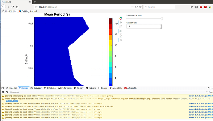
plot output in web browser
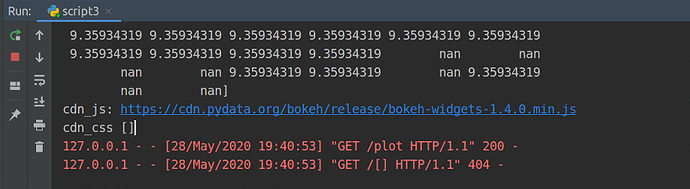
CLI
I don’t know how to change my code or add callback function show that i get the dynamic property, i think i have to use Torando but how to change code that i don’t know
I am using windows Operating system.
Thank you.