Slow performance with Holoviews live data

Hi, I’m seeing slow performance with streaming data. Each update is displaying 1 hv.Bar point, hv.Curve (160 points) / hv.Image objects (160x512), and each update is taking ~68ms (14fps).

Demo notebook with dummy data: Benchmark-Live-Holoviews.ipynb · GitHub

Video of it running: Imgur: The magic of the Internet

I wonder if repeatedly creating the plot objects each time my plot function is called is slowing it down. Is it possible to update the data in the plot dynamically instead of re-creating it?

Ideally, I could simply send the latest data point on each update instead of the whole history buffer. But even if re-rendering the full buffer, it still feels like it’s unreasonably slow. Any ideas on how to make this faster?

More details: I’m on an 8-core 2019 MacBook Pro. The use case is to plot a live spectrogram, showing a rolling 5 seconds of audio (30Hz data, 512 bins of data) and some stats about it.

I get ~17fps when running as a Panel app without the ipywidgets.

I don’t know what to expect. 60fps would be really awesome. But my guess is also that alternative data app frameworks cannot deliver anything like 17fps?

import numpy as np
import holoviews as hv
from holoviews import opts
import time

hv.extension("bokeh", logo=False)

FRAMES = 160
N_BINS = 512
spec_buffer = np.zeros((N_BINS, FRAMES))
activation_buffer = np.zeros(FRAMES)

last = time.time()

def plot_fn(data):
    global last
    now = time.time()
    elapsed, last = now - last, now
    fps = 1 / elapsed
    print("%.2f fps" % fps)

    if data:
        n_frames = data['spectrogram'].shape[1]
        # Rolling buffer of data
        spec_buffer[:,:-n_frames] = spec_buffer[:,n_frames:]
        spec_buffer[:,-n_frames:] = data['spectrogram']
        activation_buffer[:-n_frames] = activation_buffer[n_frames:]
        activation_buffer[-n_frames:] = data['activation']
    
    fpsbar = hv.Bars(
        ('fps', fps),
        kdims='n1',
        vdims=hv.Dimension('fps', range=(0,60)),
    ).opts(opts.Bars(width=1000, height=70, invert_axes=True))
    
    specgram = hv.Image(
        np.flip(spec_buffer, axis=0),
        bounds=(0, 0, FRAMES, N_BINS),
        kdims=[hv.Dimension("frame"), hv.Dimension("freq")]
    ).opts(opts.Image(cmap='fire', colorbar=True, tools=['hover'], width=1000, height=300))
    
    curve = hv.Curve(
        activation_buffer,
        kdims=hv.Dimension("frame"),
        vdims=hv.Dimension('activation', range=(0,1))
    ).opts(opts.Curve(width=1000, height=300))
    
    return (fpsbar + specgram + curve).cols(1)

pipe = hv.streams.Pipe()
plot = hv.DynamicMap(plot_fn, streams=[pipe])

import panel as pn
pn.extension()
pn.panel(plot).servable()
run_button = pn.widgets.Button(name="Run").servable()

@pn.depends(run_button, watch=True)
def run(_):
    iters = 100
    start = time.time()
    for i in range(iters):
        pipe.send(data={
            'spectrogram': np.random.rand(N_BINS, 1),
            'activation': np.random.rand(1),
        })
    print(f"{100 / (time.time() - start):.2f} fps average")

1 Like

You can try to profile the application as described in Performance and Debugging — Panel v0.14.2.

import numpy as np
import holoviews as hv
from holoviews import opts
import time

hv.extension("bokeh", logo=False)

FRAMES = 160
N_BINS = 512
spec_buffer = np.zeros((N_BINS, FRAMES))
activation_buffer = np.zeros(FRAMES)

last = time.time()

def plot_fn(data):
    global last
    now = time.time()
    elapsed, last = now - last, now
    fps = 1 / elapsed
    print("%.2f fps" % fps)

    if data:
        n_frames = data['spectrogram'].shape[1]
        # Rolling buffer of data
        spec_buffer[:,:-n_frames] = spec_buffer[:,n_frames:]
        spec_buffer[:,-n_frames:] = data['spectrogram']
        activation_buffer[:-n_frames] = activation_buffer[n_frames:]
        activation_buffer[-n_frames:] = data['activation']
    
    fpsbar = hv.Bars(
        ('fps', fps),
        kdims='n1',
        vdims=hv.Dimension('fps', range=(0,60)),
    ).opts(opts.Bars(width=1000, height=70, invert_axes=True))
    
    specgram = hv.Image(
        np.flip(spec_buffer, axis=0),
        bounds=(0, 0, FRAMES, N_BINS),
        kdims=[hv.Dimension("frame"), hv.Dimension("freq")]
    ).opts(opts.Image(cmap='fire', colorbar=True, tools=['hover'], width=1000, height=300))
    
    curve = hv.Curve(
        activation_buffer,
        kdims=hv.Dimension("frame"),
        vdims=hv.Dimension('activation', range=(0,1))
    ).opts(opts.Curve(width=1000, height=300))
    
    return (fpsbar + specgram + curve).cols(1)

pipe = hv.streams.Pipe()
plot = hv.DynamicMap(plot_fn, streams=[pipe])

import panel as pn
pn.extension()
pn.panel(plot).servable()
run_button = pn.widgets.Button(name="Run").servable()

@pn.depends(run_button, watch=True)
@pn.io.profile('run')
def run(_):
    iters = 100
    start = time.time()
    for i in range(iters):
        pipe.send(data={
            'spectrogram': np.random.rand(N_BINS, 1),
            'activation': np.random.rand(1),
        })
    print(f"{100 / (time.time() - start):.2f} fps average")
pip install pyinstrument snakeviz
panel serve script.py --admin --profiler=snakeviz

After clicking the run button it looks like the majority of the time is spent in BarPlot.update_frame.

1 Like

I would recommend experimenting with the Buffer. The documentation states its quite powerful and that it allows sending only the latest data to the frontend.

https://holoviews.org/user_guide/Streaming_Data.html#buffer

And then look into async as well.

https://holoviews.org/user_guide/Streaming_Data.html#asynchronous-updates-using-the-tornado-ioloop

This is awesome, thanks for the great number of pointers. I would indeed like to get to 60fps. In addition to throughput, latency is also important to me although I’m not sure how to measure that.

I think a pure JS solution could achieve much higher framerates, as right now the Python side seems to be the limiting factor (I imagine the python loop would execute much faster if it was bound by the JS side?). The Buffer optimization you mention sounds promising, I will let you know what I find.

1 Like

I stripped down the example a bit more, leaving just a single hv.Image.

Unfortunately Buffer actually makes it far slower (5fps).

FRAMES = 160
N_BINS = 512

spec_buffer = hv.streams.Buffer(
    np.random.rand(FRAMES, N_BINS),
    length=FRAMES,
    index=False
)

def spec_cb(data):
    return hv.Image(data, bounds=(0, 0, FRAMES, N_BINS))

hv.DynamicMap(spec_cb, streams=[spec_buffer])


from pyinstrument import Profiler
profiler = Profiler()
profiler.start()

iters = 10
start = time.time()
last = start
for i in range(iters):
    spec_buffer.send(np.random.rand(1, N_BINS))
    now = time.time()
    last = now
print(f"{iters / (time.time() - start):.2f} fps average")

profiler.stop()
profiler.print()
profiler.open_in_browser()

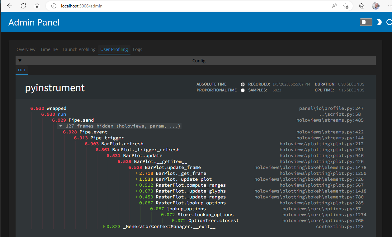
pyinstrument shows it spending most of the time in push(), JSON encoding and some sort of diffing.

Next, I ran a minimal example with Pipe.

FRAMES = 160
N_BINS = 512

rolling_buffer = np.zeros((N_BINS, FRAMES))

def spec_pipe_cb2(data):
    if data is not None:
        rolling_buffer[:,:-1] = rolling_buffer[:,1:]
        rolling_buffer[:,-1:] = data

    return hv.Image(
        rolling_buffer,
        bounds=(0, 0, FRAMES, N_BINS)
    )

spec_pipe = hv.streams.Pipe()
hv.DynamicMap(spec_pipe_cb2, streams=[spec_pipe])

iters = 100
start = time.time()
last = start
for i in range(iters):
    spec_pipe.send(np.random.rand(N_BINS, 1))
    now = time.time()
    last = now
print(f"{iters / (time.time() - start):.2f} fps average")

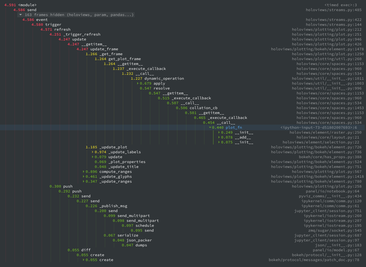
It runs at 47fps, which is pretty good. However as soon as I add a second plot with a Curve it goes to 27fps. It’s only spending 9% of time in my Pipe callback but everything it does afterwards is immense.

I may next try to use Bokeh directly (without Holoviews) for this real-time use case.

I will say that the performance is a bit noticeable in other situations as well; for example I needed to render 30-40 small plots side-by-side and it took a noticeable amount of time, and with ~300 plots and it was taking upwards of 30 seconds.

A quick update on this. The Bokeh-based approach was indeed much faster.

The fps is somewhere between 55-100fps. The in-notebook timing is not accurate as the data gets queued up to be sent asynchronously and the notebook cell completes executing before all the data is sent. I’m just estimating fps based on when the graph finishes updating. But, this is good enough for my needs now.

In a Jupyter notebook:

import time
from bokeh.plotting import figure
import panel as pn
import numpy as np
pn.extension()

TIME_RANGE = 5.15
FRAMES = 160
N_BINS = 512

spec_buffer = np.random.rand(N_BINS, FRAMES)
activation_buffer = np.random.rand(FRAMES)

OPTS = dict(plot_width=800, plot_height=300,
              tools="xpan,reset,save,xwheel_zoom",
              x_range=[-TIME_RANGE, 0],
           )

fig1 = figure(**OPTS, title="spectrogram", y_range=[0, N_BINS])
spec_plot = fig1.image([spec_buffer], x=-TIME_RANGE, y=0, dw=TIME_RANGE, dh=N_BINS)

fig2 = figure(**OPTS, title="activation", y_range=[0, 1])
act_plot = fig2.line(np.linspace(-TIME_RANGE, 0, FRAMES), activation_buffer)

pane = pn.Pane(pn.Column(fig1, fig2))

def shift_in(target, src):
    n = src.shape[-1]
    target[..., :-n] = target[..., n:]
    target[..., -n:] = src

pane
%%time

iters = 500
start = time.time()
last = start
for i in range(iters):
    shift_in(spec_buffer, np.random.rand(N_BINS, 1))
    shift_in(activation_buffer, np.random.rand(1))
    
    spec_plot.data_source.data['image'] = [spec_buffer]
    act_plot.data_source.data['y'] = activation_buffer
    pn.io.push_notebook(pane)
    
    now = time.time()
    last = now
print(f"{iters / (time.time() - start):.2f} fps average")
2 Likes