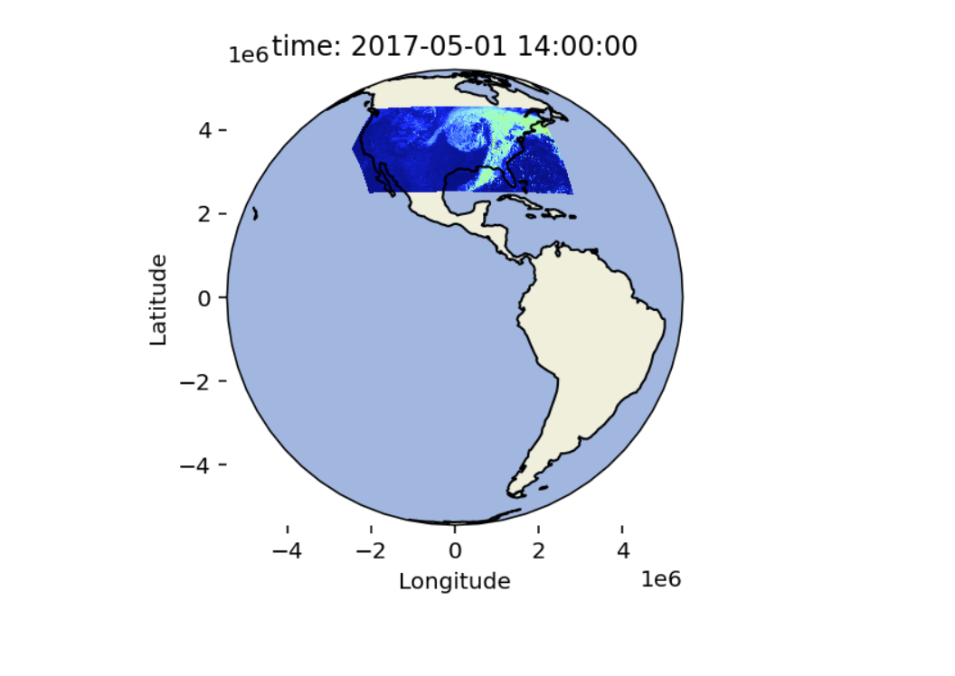
I have been plotting some gridded satellite data using the Geoviews Image and matplotlib backend. The data is already in a plate carree projection. I have successfully plotted the data in plate carree, lambert cylindrical, and Mercator projections. These plots look correct, and the axis are labeled with the proper lat/lon coordinates. However any time I apply a projection that is rounded (orthographic, mollewide, or geostationary) the resulting plot looks correct, but the axis values are no longer in lat/lon coordinates. I attached a screenshot below of my geostationary plot with the unknown axis values. All of the rounded/globe projections I have tried plot the image in the correct location but the axis always seems to be in scientific notation. I am unsure if this is correct, but I thought maybe the scientific coordinates showing on the axis were the coordinates created when switching from plate carree to another projection. I also seemed to notice a lot of the examples in the gallery and documentation that used globe projections had the axes turned off. Is there anyway I can show the projections with the original lat/lon coordinates associated with the data?
Hi @sbail
Welcome to the community.
Please provide a minimum, reproducible code example. It will make it much easier for the community to try to help. Thanks.
I think those are projected coordinates; similar to eastings/northings for Mercator.
Maybe you can overlay graticules:
https://geoviews.org/user_guide/Geometries.html
gv.output(backend='bokeh')

(gf.ocean * gf.land.options(scale='110m', global_extent=True) * gv.Feature(graticules, group='Lines') +
 gf.ocean * gf.land.options(scale='50m', global_extent=True) * gv.Feature(graticules, group='Lines'))
and maybe there’s a group=‘Labels’?
Reproducible example:
ds = xr.open_mfdataset(“C:/Users/SydneyBailey/Documents/IRAD503/GridSat3Hour/*.nc”, concat_dim=‘time’, combine=‘nested’, parallel=True)
kdims = [‘time’, ‘lat’, ‘lon’]
vdims = [ ‘ch6’ ]
xr_dataset = gv.Dataset(ds, kdims=kdims, vdims=vdims, crs= crs.PlateCarree())
#creates plate carree projection w/ correct lat/lon on axis
gf.ocean * gf.land * (xr_dataset.to.image([‘lon’, ‘lat’]) * gf.coastline).opts(
opts.Image(projection=crs.PlateCarree(), fig_size=200))
#creates plot above with different values on axis
img = xr_dataset.to.image([‘lon’, ‘lat’])
gf.land * gf.ocean * img.opts(cmap=‘jet’,
projection=crs.Geostationary(central_longitude=ds[‘lon’].values.mean()),
global_extent=True) * gf.coastline