I’ve tried using both gv.Shape.from_records() and hvplot.pandas and both seem to halt interactivity after I launch a panel app. Is there a third way that I’m missing?
Here’s some sample code of mine:
import panel as pn
import xarray as xr
import hvplot.xarray
import hvplot.pandas

shp = gpd.read_file("/Users/james/Downloads/cb_2018_us_county_500k/cb_2018_us_county_500k.shp")

ds = xr.open_dataset("http://basin.ceoe.udel.edu/thredds/dodsC/DEOSRefET.nc")
df = ds.refET[0]

df.hvplot.quadmesh(width=500, height=1000, x='longitude', y='latitude', project=True, geo=True,
             rasterize=True, dynamic=False) * shp.hvplot(geo=True, color=None)
I’m trying to use panel to visualize this dataset but figured it would be best to start out with the general holoviews code I’m basing the panel code off of. I can attach my full code if necessary.
1 Like
I’ve found through trial and error that the most efficient way to overlay a shapefile onto a hvplot.xarray quadmesh plot is via cartopy and geoviews. An important note that was helpful was clipping the shapefile to a much smaller domain that fit my data before overlaying it on the image. I did this using GDAL’s ogr2ogr. Once the file was clipped, I used cartopy.io.shapereader to load in a shapefile and then use geoviews.Shape.from_records(). Once it’s a geoviews.Shape object, I convert it to a geoviews.Polygon object for overlay. Below is an example:
import panel as pn
import xarray as xr
import hvplot.xarray
import hvplot.pandas
import cartopy.io.shapereader as shpreader

state_lines = shpreader.Reader("/Users/James/Downloads/cb_2018_us_state_500k/" + 'cb_2018_us_state_500clipped.shp')
state_lines = gv.Shape.from_records(state_lines.records())
shp = gv.Polygons(state_lines).opts('Polygons', line_color='black',fill_color=None)

ds = xr.open_dataset("http://basin.ceoe.udel.edu/thredds/dodsC/DEOSRefET.nc")
df = ds.refET[0]

df.hvplot.quadmesh(width=500, height=1000, x='longitude', y='latitude', project=True, geo=True,
             rasterize=True, dynamic=False) * shp
Sorry I never responded here, the most efficient approach should definitely be what you tried first and if that doesn’t work we should track down the reason so an issue would be good.
This is still a problem Mr. @philippjfr You can replicate the issue with
import hvplot.pandas
import hvplot.xarray
import geopandas as gpd
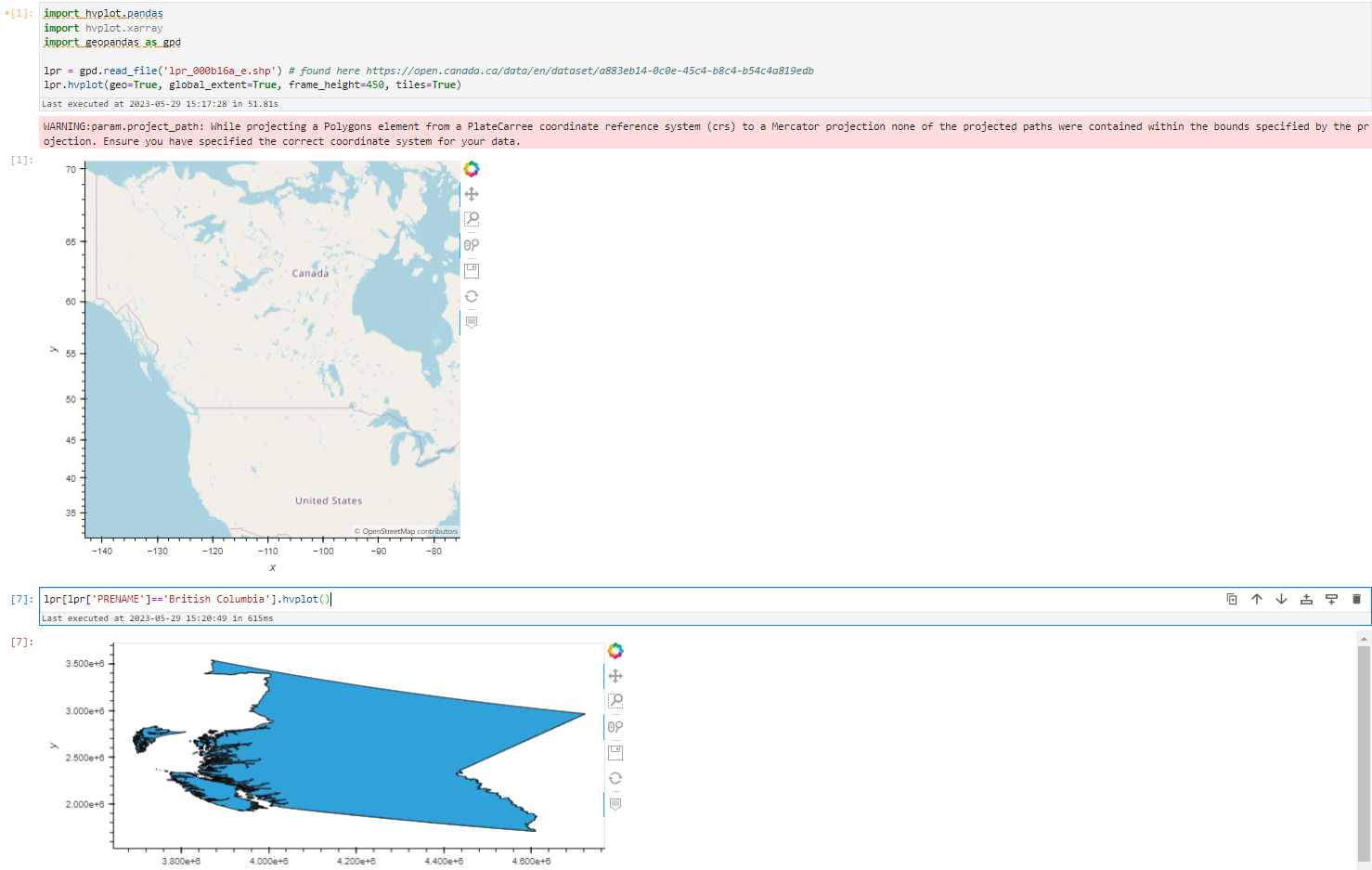
lpr = gpd.read_file('lpr_000b16a_e.shp') # found here https://open.canada.ca/data/en/dataset/a883eb14-0c0e-45c4-b8c4-b54c4a819edb
lpr.hvplot(geo=True, global_extent=True, frame_height=450, tiles=True)
lpr[lpr['PRENAME']=='British Columbia'].hvplot()
takes almost a minute and this is what I see
Using :
pandas - [ 2.0.1 ]
hvplot - [ 0.8.3 ]
panel - [ 0.14.4 ]
geopandas - [ 0.12.2 ]
Partial workaround :
import hvplot.pandas
import geopandas as gpd
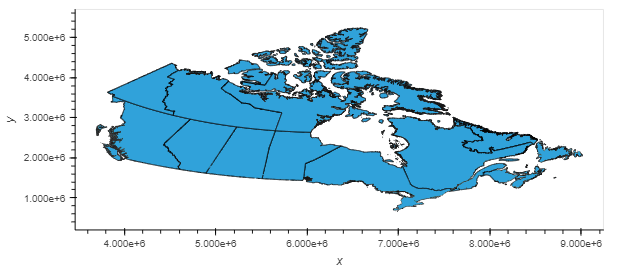
lpr = gpd.read_file('lpr_000b16a_e.shp', driver="ESRI Shapefile") # found here https://open.canada.ca/data/en/dataset/a883eb14-0c0e-45c4-b8c4-b54c4a819edb
lpr.hvplot()
this takes 15.46s and produces
How big is the file? If you have to send a lot of data to the browser, it will always be a problem.
It’s a 52Mb shapefile Mr. @Hoxbro . If you know of a better way to have higher resolution provinces (or even more) equivalent to coastline features that do not slow down the app to a crawl that would be great!