@ahuang11 I also would guess it’s something related to the chunk size but I don’t understand why the chunk size is different if using daskobj.hvplot.scatter(). The reference gallery entry for hvplot Scatter does not mention chunk size. Not sure where it should be defined… ![]()
@philippjfr I’ll try that. First I update the MWE do it is possible to use it with the dask dashboard. Here is updated code:
Updated MWE
Updated MWE
This time it is in form for installable package:
📁 panel-mwe/
├─📁 myproj/
│ ├─📄 app.py
│ ├─📄 task.py
│ └─📄 __init__.py   # empty file
└─📄 pyproject.toml
pyproject.toml
[project]
name = "myproj"
description = "myproj"
version = "0.1.0"
dependencies = [
    "dask[distributed]",
    "panel",
    "hvplot",
    "pyarrow",
]

[build-system]
build-backend = "flit_core.buildapi"
requires = ["flit_core >=3.2,<4"]
myproj/app.py
from __future__ import annotations


import dask.dataframe as dd
from dask.distributed import Client
import hvplot.dask  # noqa
import hvplot.pandas # noqa
import panel as pn

import sys

from myproj.task import get_data, get_mae


@pn.cache
def get_dask_client() -> Client:
    client = Client("tcp://127.0.0.1:8786")
    return client


def create_graph(
    file: str,
    minute_of_day: tuple[float, float],
    identifiers: list[int],
):
    client = get_dask_client()
    minute_of_day = tuple(map(round, minute_of_day))

    mae_a = client.submit(
        get_mae,
        file=file,
        minute_of_day=minute_of_day,
        identifiers=identifiers,
        label="A",
    ).result()
    mae_b = client.submit(
        get_mae,
        file=file,
        minute_of_day=minute_of_day,
        identifiers=identifiers,
        label="B",
    ).result()

    common_opts = dict(legend="top")
    graph_scatter_pipeline = mae_b.hvplot.scatter(
        label="B", **common_opts
    ) * mae_a.hvplot.scatter(label="A", **common_opts)

    return graph_scatter_pipeline


pn.param.ParamMethod.loading_indicator = True
pn.extension(sizing_mode="stretch_width", throttled=True)


minute_of_day = pn.widgets.RangeSlider(
    name="Minute of day", start=0, end=1440, value=(0, 1440), step=10
)
unique_ids = [21, 79]
identifiers = pn.widgets.MultiChoice(
    name="Identifiers", options=unique_ids, value=unique_ids
)
imain_graph = pn.bind(
    create_graph, file=sys.argv[1], minute_of_day=minute_of_day, identifiers=identifiers
)
main_graph = pn.panel(imain_graph)

minute_of_day.servable(area="sidebar")
identifiers.servable(area="sidebar")
main_graph.servable(title="Data graph")
myproj/task.py
from __future__ import annotations

import dask.dataframe as dd
import panel as pn


@pn.cache
def get_data(file) -> dd.DataFrame:
    df = dd.read_parquet(file)
    for i in range(15):
        df[f"extra_col{i}"] = df["val_A"] + i
    return df


def get_mae(
    file: str,
    minute_of_day: tuple[int, int],
    identifiers: list[int],
    label: str,
) -> dd.Series:
    df = get_data(file)
    df_filtered = _filter_based_on_ui_selections(
        df, minute_of_day=minute_of_day, identifiers=identifiers
    )
    mae = do_calculate_mae(df_filtered, label=label)
    return mae


def _filter_based_on_ui_selections(
    df: dd.DataFrame,
    minute_of_day: tuple[int, int],
    identifiers: list[int],
) -> dd.DataFrame:
    df_filtered = df[df["minute_of_day"].between(*minute_of_day)]
    return df_filtered[df_filtered["identifier"].isin(identifiers)]


def do_calculate_mae(
    df: dd.DataFrame,
    label: str,
) -> dd.Series:
    col_err = f"err_{label}"
    df[col_err] = abs(df[f"val_{label}"] - df["val_C"])
    mae = df.groupby("minute_of_day")[col_err].agg("mean")

    return mae
Commands
Setting up: Create a virtual environment, activate it, and install the myproj. Run in the project root (same folder with pyproject.toml)
python -m venv venv
source venv/bin/activate
python -m pip install -e .
Starting:
First, start the dask scheduler and a worker. These need to be ran in separate terminal windows, and both need to have the virtual environment activated (+any changes to the app require restarting both of these)
dask scheduler --host=tcp://127.0.0.1 --port=8786
dask worker tcp://127.0.0.1:878
then start the panel app:
python -m panel serve myproj/app.py --show --admin --args ~/Downloads/testdata.parquet
The data file link is in the first post.
MWE results
I’m using more powerful computer than in the OP. Here only one worker on dask.
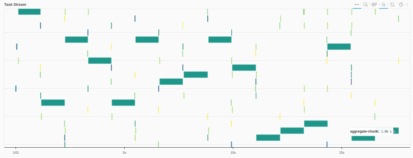
Using daskobj.hvplot.scatter:
code
    # mae_a and mae_b are dask series
    graph_scatter_pipeline = mae_b.hvplot.scatter(
        label="B", **common_opts
    ) * mae_a.hvplot.scatter(label="A", **common_opts)
results
- Initial load 19 seconds, filtering ~14 seconds

- one task (initial load, filtering) looks like this
Using pandasobj.hvplot.scatter:
Add a .compute() to convert dask serie to pandas serie:
code changes
    mae_a = (
        client.submit(
            get_mae,
            file=file,
            minute_of_day=minute_of_day,
            identifiers=identifiers,
            label="A",
        )
        .result()
        .compute() #here
    )
    mae_b = (
        client.submit(
            get_mae,
            file=file,
            minute_of_day=minute_of_day,
            identifiers=identifiers,
            label="B",
        )
        .result()
        .compute() #here
    )

    common_opts = dict(legend="top")
    graph_scatter_pipeline = mae_b.hvplot.scatter(
        label="B", **common_opts
    ) * mae_a.hvplot.scatter(label="A", **common_opts)
results
About 10 seconds for page load, and 2-3 seconds for filtering
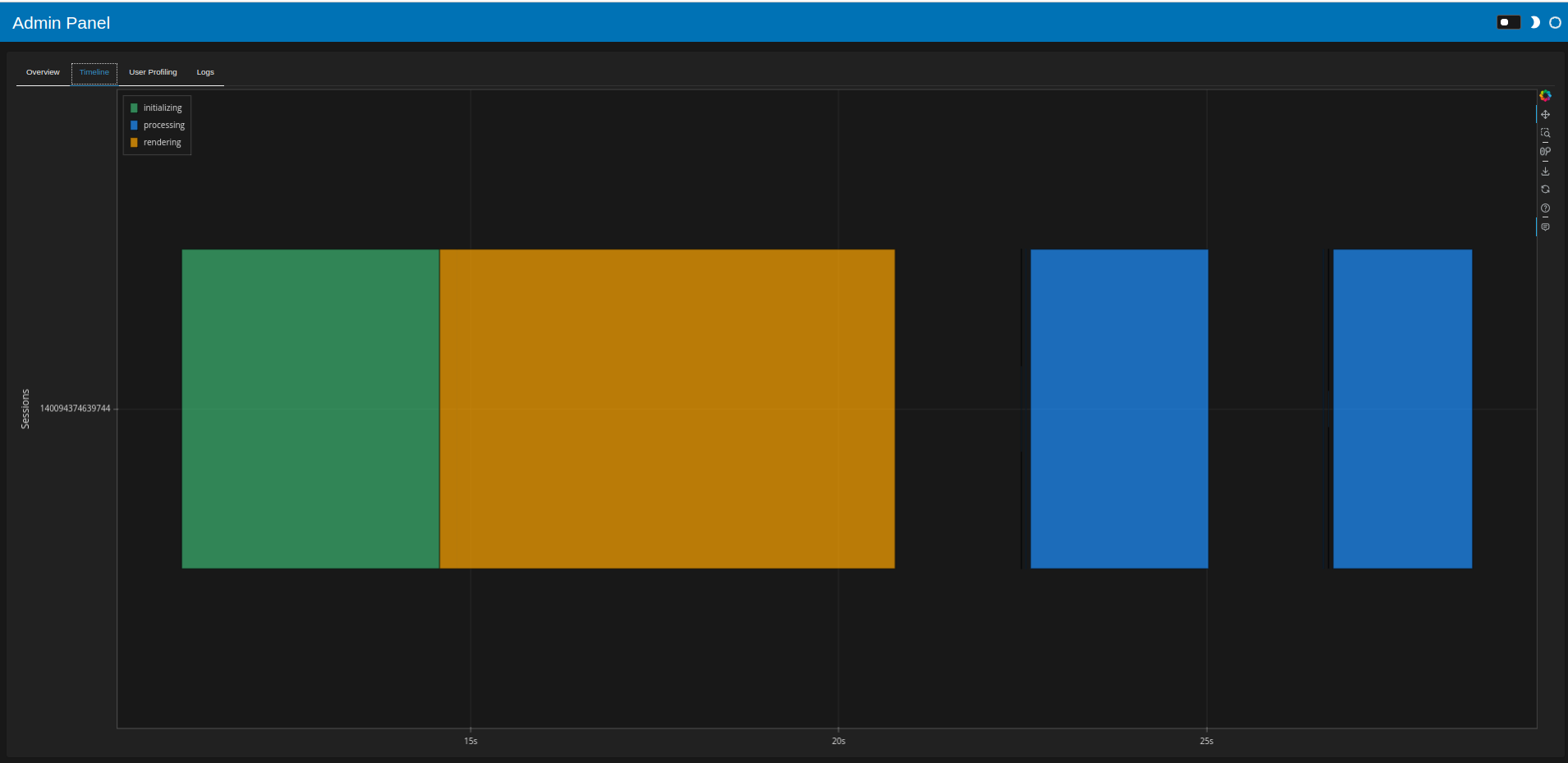
The dask Task Stream looks much better. Each task (initial load, filtering) produces something like this:
The daskobj.persist().hvplot.scatter
code changes
    mae_a = client.submit(
        get_mae,
        file=file,
        minute_of_day=minute_of_day,
        identifiers=identifiers,
        label="A",
    ).result()
    mae_b = client.submit(
        get_mae,
        file=file,
        minute_of_day=minute_of_day,
        identifiers=identifiers,
        label="B",
    ).result()

    common_opts = dict(legend="top")
    graph_scatter_pipeline = mae_b.persist().hvplot.scatter( # persists here
        label="B", **common_opts
    ) * mae_a.persist().hvplot.scatter(label="A", **common_opts)
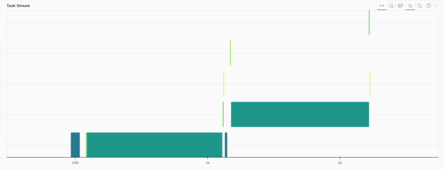
results
Speed from the panel admin:
- 8 sec initial load
- About 2 seconds to filter afterwards
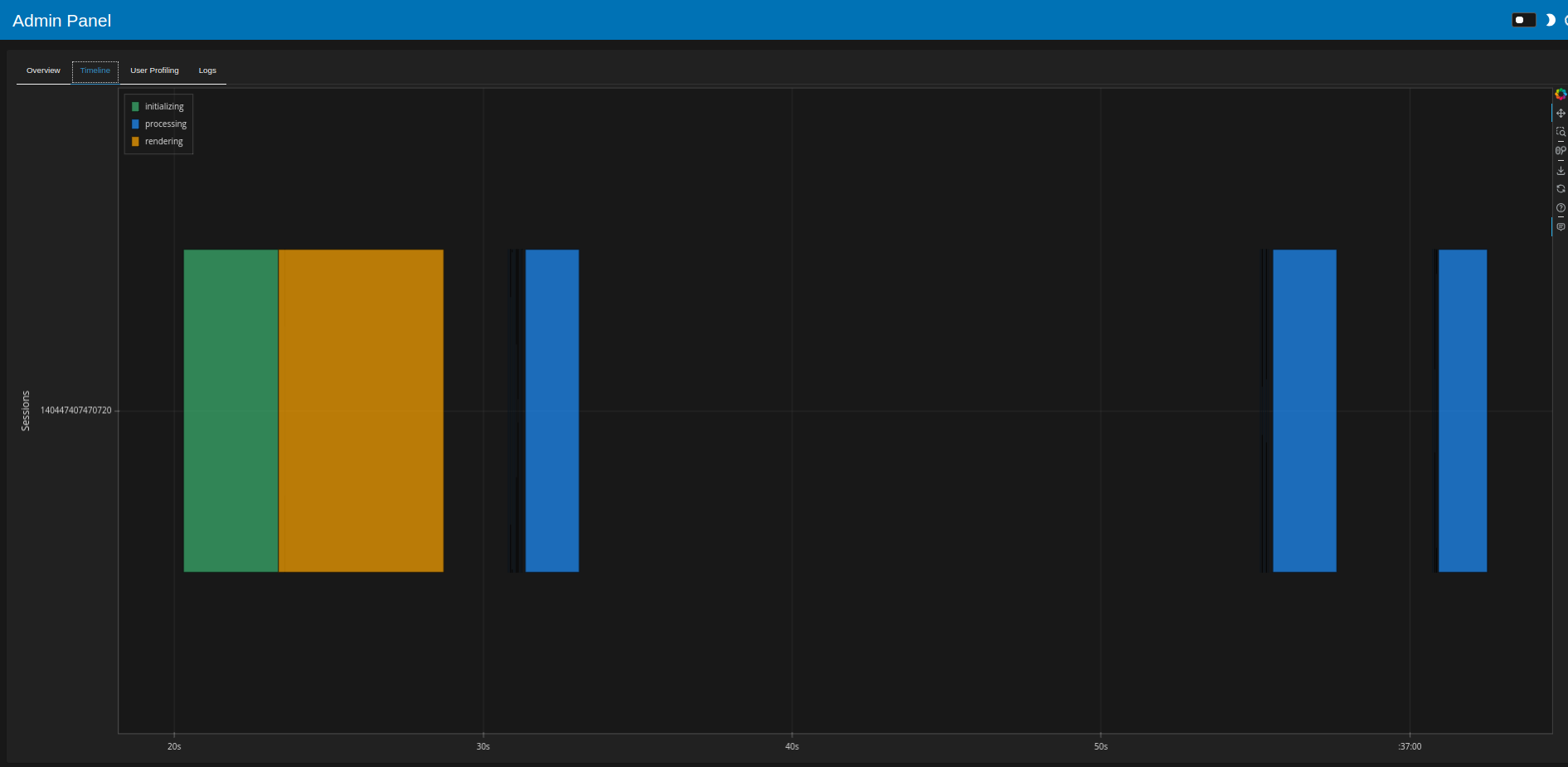
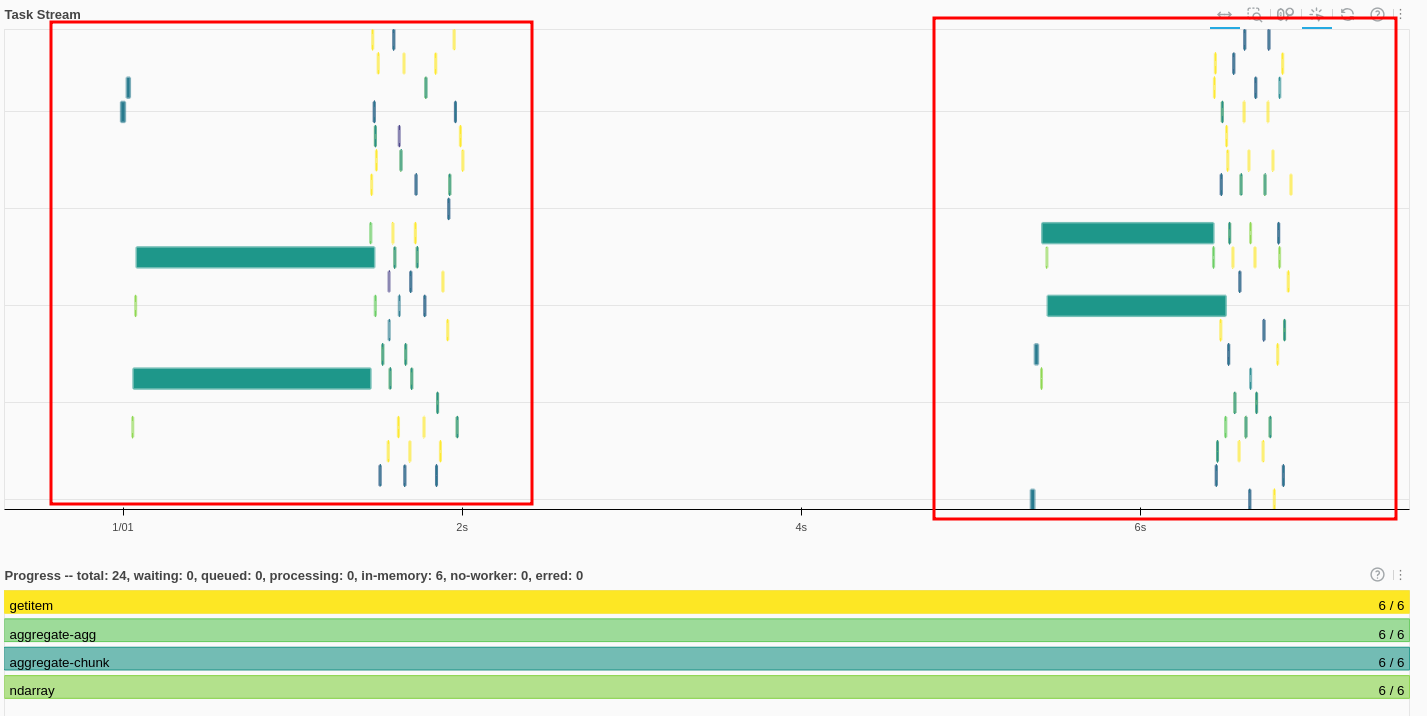
Initial page load and filtering produce something like this in the dask dashboard:
Reference: using only pandas

Summary of results
- pandas only: 4 sec initial load, 1-2 sec filtering
- dask + dask.hvpot: 19 sec initial load, 14 sec filtering
- dask.compute() + pandas.hvplot: 10 sec initial load, 2-3 sec filtering
- dask + dask.persist().hvplot: 8 sec initial load, 2 sec filtering