Why Panel is 10x slower with Dask than with Pandas?

fohrloop · January 22, 2024, 3:26pm

I have an application which should

Read raw data (ultimately, 100’s of millions of rows)
Filter data based on widgets
Draw graphs

I’m evaluating Holoviz for the purpose. Now I have created an application which uses Dask, but it’s really, really slow. I’ve tried to reproduce the slowness in this MWE app with a dummy data set.

Code for MWE app:

from __future__ import annotations

import sys

import dask.dataframe as dd
import hvplot.dask  # noqa
import panel as pn


@pn.cache
def get_data() -> dd.DataFrame:
    df = dd.read_parquet(sys.argv[1])
    for i in range(15):
        df[f"extra_col{i}"] = df["val_A"] + i
    return df


def create_graph(
    df: dd.DataFrame,
    minute_of_day: tuple[float, float],
    identifiers: list[int],
):

    minute_of_day = tuple(map(round, minute_of_day))

    mae_a = calculate_mae(
        df=df,
        label="A",
        minute_of_day=minute_of_day,
        identifiers=identifiers,
    )
    mae_b = calculate_mae(
        df=df,
        label="B",
        minute_of_day=minute_of_day,
        identifiers=identifiers,
    )

    common_opts = dict(legend="top")
    graph_scatter_pipeline = mae_b.hvplot.scatter(
        label="B", **common_opts
    ) * mae_a.hvplot.scatter(label="A", **common_opts)

    return graph_scatter_pipeline


def calculate_mae(
    df: dd.DataFrame,
    minute_of_day: tuple[int, int],
    identifiers: list[int],
    label: str,
) -> dd.Series:
    df_filtered = _filter_based_on_ui_selections(
        df, minute_of_day=minute_of_day, identifiers=identifiers
    )
    mae = do_calculate_mae(df_filtered, label=label)
    return mae


def _filter_based_on_ui_selections(
    df: dd.DataFrame,
    minute_of_day: tuple[int, int],
    identifiers: list[int],
) -> dd.DataFrame:

    df_filtered = df[df["minute_of_day"].between(*minute_of_day)]
    return df_filtered[df_filtered["identifier"].isin(identifiers)]


def do_calculate_mae(
    df: dd.DataFrame,
    label: str,
) -> dd.Series:

    col_err = f"err_{label}"
    df[col_err] = abs(df[f"val_{label}"] - df["val_C"])
    mae = df.groupby("minute_of_day")[col_err].agg("mean")

    return mae


pn.param.ParamMethod.loading_indicator = True
pn.extension(sizing_mode="stretch_width", throttled=True)


dfraw = get_data()
df = dfraw.interactive()

minute_of_day = pn.widgets.RangeSlider(
    name="Minute of day", start=0, end=1440, value=(0, 1440), step=10
)
unique_ids = list(dfraw["identifier"].unique())
identifiers = pn.widgets.MultiChoice(
    name="Identifiers", options=unique_ids, value=unique_ids
)
imain_graph = pn.bind(
    create_graph, df, minute_of_day=minute_of_day, identifiers=identifiers
)
main_graph = pn.panel(imain_graph)

minute_of_day.servable(area="sidebar")
identifiers.servable(area="sidebar")
main_graph.servable(title="Data graph")

Running the code

 python -m panel app.py --autoreload --show --args [data_file]

Test data

The data_file is testdata.parquet from here, and for possible link rot, the data looks like this:

>>> df.head()
   identifier     val_A     val_B  minute_of_day     val_C
0          79  0.171269  0.254808            780  0.225462
1          79 -0.094295  0.041287            780 -0.037825
2          79  0.138048  0.075044            790  0.114881
3          21 -0.206397 -0.229667            310 -0.147015
4          21 -0.185620 -0.236410           1080 -0.196957

identifier is random id. Now there is only 21 and 79
minute_of_day is integer 0 <= x <= 1440
val_A, val_B and val_C are random numbers (from random walkers).
about 5 million rows.

Edit: Additional Benchmarks

The data processing part takes (see below):

with pandas only about 1.5 seconds
with pandas + Panel about 3 seconds
with Dask only about 3 seconds (some overhead cost using Dask is understandable)
with Dask + Panel about 30 seconds

Question

Why is the app so slow and what could be done to make it faster? This one is slow even with the ~5 million data points fake dataset. The real app obviously has more calculations, more filtering and is even slower. I’m clearly missing something as I’ve under the impression a Panel app could handle easily datasets with hundreds of millions of rows.

ahuang11 · January 22, 2024, 5:22pm

Some random suggestions:

try caching (pn.cache)
try loading data after server loads (pn.state.onload)
check out Scaling with Dask — Panel v1.3.7

fohrloop · January 23, 2024, 10:13am

Thank you @ahuang11 for the suggestions.

caching: I have already enabled pn.cache for getting the data, but I could improve by adding caching for getting the list of identifiers.
I wasn’t aware of the pn.state.onload, I will try to utilize it, thanks!
Scaling with Dask: Another good tip! I’ll definitely try to use the tricks from the linked page once I try my 500M row dataset! I’ll just first try to get the performance right with the smaller dataset. I could also check pandas if that’s faster with the small dataset.

fohrloop · January 23, 2024, 10:21am

Profiling (app using Dask)

I’m trying to see where the time is used. I followed the instructions about debugging and enabled the admin panel with profiling on the only pn.bind decorated function. Here are the admin panel results:

1: initialization of the dashboard. Takes 30 seconds. Not a show stopper.
2,3,4 & 5: The blue boxes are all 20-31 seconds. They show how much wait time there is after I use the slider widget. This much slower than anticipated.

The profiling code

Added pn.io.profile to the only callback in the application.
If I have understood correctly, this is the only thing that is called after widgets are touched. Is that so?

@pn.io.profile("formatting", engine="snakeviz")
def create_graph(
    df: dd.DataFrame,
    minute_of_day: tuple[float, float],
    identifiers: list[int],
):

Profiling results

Here are the results, which to me do not make any sense to me. The time for create_graph was accumulated roughly 0.16 seconds per each callback call (did it four times to get to 0.625 seconds).
This does not add up: If the functions takes 0.625 seconds to execute, why the processing time is 30 seconds? I wonder if this is because of Dask or because time is used somewhere in the JavaScript world…?

fohrloop · January 23, 2024, 10:31am

Profiling with pandas

Same test as above, but by using pandas instead of Dask

1: initialization of the dashboard. Takes 4 seconds. (Dask took 30 seconds with same dataset)
2,3,4 & 5: The blue boxes are all 1-3 seconds. They show how much wait time there is after I use the slider widget. Compare to the 20-30 seconds used by Dask.

Profiling results

The same results, but now using pandas instead of Dask.
Now the results add up. The total time used by the bound function create_graph was 6.3 seconds, which is at roughly the sum of all the blue “processing” boxes above.

Summary

Most of the time is definitely used by Dask
The @pn.io.profile does not work with Dask, and I assume it is because Dask dataframe operations are lazily evaluated. But to profile Panel apps which use Dask, then?

fohrloop · January 23, 2024, 11:11am

I just did some testing and noticed that something is making Dask to consume 10x more time with Panel vs. without Panel

The data processing part takes:

with pandas only about 1.5 seconds
with pandas + Panel about 3 seconds
with Dask only about 3 seconds (some overhead cost using Dask is understandable)
with Dask + Panel about 30 seconds

Reproducable example showing that Dask takes only 3 seconds to process the data

Use the same testdata.parquet as in previous posts in this thread.
Run with python dasktest.py testdata.parquet

This prints out

get_data: 0.12 s
create_data_for_graph: 0.03 s
compute: 3.18 s

Code:

# dasktest.py
from __future__ import annotations

import sys
import dask.dataframe as dd
import time

import panel as pn


@pn.cache
def get_data() -> dd.DataFrame:
    df = dd.read_parquet(sys.argv[1])
    for i in range(15):
        df[f"extra_col{i}"] = df["val_A"] + i
    return df


def create_data_for_graph(
    df: dd.DataFrame,
    minute_of_day: tuple[float, float],
    identifiers: list[int],
):

    minute_of_day = tuple(map(round, minute_of_day))

    mae_a = calculate_mae(
        df=df,
        label="A",
        minute_of_day=minute_of_day,
        identifiers=identifiers,
    )
    mae_b = calculate_mae(
        df=df,
        label="B",
        minute_of_day=minute_of_day,
        identifiers=identifiers,
    )

    return mae_a, mae_b


def calculate_mae(
    df: dd.DataFrame,
    minute_of_day: tuple[int, int],
    identifiers: list[int],
    label: str,
) -> dd.Series:
    df_filtered = _filter_based_on_ui_selections(
        df, minute_of_day=minute_of_day, identifiers=identifiers
    )
    mae = do_calculate_mae(df_filtered, label=label)
    return mae


def _filter_based_on_ui_selections(
    df: dd.DataFrame,
    minute_of_day: tuple[int, int],
    identifiers: list[int],
) -> dd.DataFrame:

    df_filtered = df[df["minute_of_day"].between(*minute_of_day)]
    return df_filtered[df_filtered["identifier"].isin(identifiers)]


def do_calculate_mae(
    df: dd.DataFrame,
    label: str,
) -> dd.Series:

    col_err = f"err_{label}"
    df[col_err] = abs(df[f"val_{label}"] - df["val_C"])
    mae = df.groupby("minute_of_day")[col_err].agg("mean")

    return mae


t0 = time.time()
df = get_data()
t_get_data = time.time()
mae_a, mae_b = create_data_for_graph(df, minute_of_day=(0, 1440), identifiers=[21, 79])
t_create_data_for_graph = time.time()
mae_a = mae_a.compute()
mae_b = mae_b.compute()
t_compute = time.time()

print(f"get_data: {t_get_data - t0:.2f} s")
print(f"create_data_for_graph: {t_create_data_for_graph - t_get_data:.2f} s")
print(f"compute: {t_compute - t_create_data_for_graph:.2f} s")
breakpoint()

Question

Why there is so much overhead added when Dask is used with Panel?

fohrloop · January 23, 2024, 12:06pm

Using .compute() before creating hvplots

I did this small change:

add daskseries.compute() to convert the Dask series to pandas Series just before creating the plots with .hvplot.scatter.

Code

@pn.io.profile("profile", engine="snakeviz")
def create_graph(
    df: dd.DataFrame,
    minute_of_day: tuple[float, float],
    identifiers: list[int],
):

    minute_of_day = tuple(map(round, minute_of_day))

    mae_a = calculate_mae(
        df=df,
        label="A",
        minute_of_day=minute_of_day,
        identifiers=identifiers,
    ).compute()         # added .compute()
    mae_b = calculate_mae(
        df=df,
        label="B",
        minute_of_day=minute_of_day,
        identifiers=identifiers,
    ).compute()         # added .compute()

    common_opts = dict(legend="top")
    graph_scatter_pipeline = mae_b.hvplot.scatter(
        label="B", **common_opts
    ) * mae_a.hvplot.scatter(label="A", **common_opts)

    return graph_scatter_pipeline

Results

The speed is now comparable to using pandas.Series (good!). The processing took now only 2-4 seconds (with pandas, took about the same).

Now I can also see the results from the profiler.
The total time used in the profiled create_graph function is about 9 seconds (3 calls x 3 seconds).
Most of the time is actually used in acquiring a lock. Edit: This is actually expected behaviour. Quotation from the dask discourse:

This is entirely expected: snakeviz/profile only looks at what your main thread is doing, but all of the compute work is happening in other threads, so it just shows “wait”. This is one of the reasons to use distributed even just locally (LocalCluster), because it gives much better diagnostic information.

I’m still wondering why the conversion from dask to pandas is required for the speedup? Isn’t Panel compatible with Dask? What I’m missing?

ahuang11 · January 23, 2024, 3:35pm

Another suggestion is checking the dask client dashboard and see what’s going on.

jerry.vinokurov · January 23, 2024, 9:50pm

Hi @fohrloop,

I have not run your exact code but from the diagnostics you have provided and the fact that calling compute brings your performance in line with what is expected, I would have to guess that there are places where your dask graph is being evaluated and then discarded, and this is happening repeatedly, which causes your slowdown. Since you have bound a widget to a function that evaluates based on that widget’s value it could be that you are triggering computations every time you drag the widget. It’s not that there’s any problematic interaction with panel as such, it’s that your actions in panel are triggering computations that then do not get materialized to the frontend and you are experiencing this as latency. If you take a look at the dask task stream, you should be able to identify which of your actions produce which computations.

fohrloop · January 24, 2024, 3:02pm

@ahuang11 , @jerry.vinokurov

My problem (for this message) is essentially solved but I’ll leave this for the future googlers. (see the Solution section)

I am trying to use a local Dask cluster and to set up the dask client dashboard.

Just Dask, no Panel

For some reason the dask code works without Panel:

# full MWE below
client = get_client()
future = client.submit(get_data_for_graph, sys.argv[1], (0, 1440), [21, 79])
mae_a, mae_b = future.result()
mae_a = mae_a.compute()
mae_b = mae_b.compute()

print(mae_a, mae_b)

printout

minute_of_day
780     0.055595
790     0.042109
310     0.046115
1080    0.031772
1170    0.030551
          ...   
210     0.052976
1160    0.039351
420     0.049656
350     0.033365
530     0.046255
Name: err_A, Length: 144, dtype: float64 minute_of_day
780     0.067251
790     0.060881
310     0.060365
1080    0.049023
1170    0.033088
          ...   
210     0.071234
1160    0.049264
420     0.079492
350     0.032884
530     0.065835
Name: err_B, Length: 144, dtype: float64

Full MWE code

This one uses the same test dataset testdata.parquet given above.

from __future__ import annotations

import sys

import dask.dataframe as dd
from dask.distributed import Client
import hvplot.dask  # noqa
import panel as pn


def get_data(file) -> dd.DataFrame:
    df = dd.read_parquet(file)
    for i in range(15):
        df[f"extra_col{i}"] = df["val_A"] + i
    return df


@pn.cache  # share the client across all users and sessions
def get_client():
    return Client("tcp://127.0.0.1:8786")


def get_data_for_graph(
    file: str,
    minute_of_day: tuple[float, float],
    identifiers: list[int],
):

    df = get_data(file)

    mae_a = calculate_mae(
        df=df,
        label="A",
        minute_of_day=minute_of_day,
        identifiers=identifiers,
    )
    mae_b = calculate_mae(
        df=df,
        label="B",
        minute_of_day=minute_of_day,
        identifiers=identifiers,
    )
    return mae_a, mae_b


def calculate_mae(
    df: dd.DataFrame,
    minute_of_day: tuple[int, int],
    identifiers: list[int],
    label: str,
) -> dd.Series:
    df_filtered = _filter_based_on_ui_selections(
        df, minute_of_day=minute_of_day, identifiers=identifiers
    )
    mae = do_calculate_mae(df_filtered, label=label)
    return mae


def _filter_based_on_ui_selections(
    df: dd.DataFrame,
    minute_of_day: tuple[int, int],
    identifiers: list[int],
) -> dd.DataFrame:

    df_filtered = df[df["minute_of_day"].between(*minute_of_day)]
    return df_filtered[df_filtered["identifier"].isin(identifiers)]


def do_calculate_mae(
    df: dd.DataFrame,
    label: str,
) -> dd.Series:

    col_err = f"err_{label}"
    df[col_err] = abs(df[f"val_{label}"] - df["val_C"])
    mae = df.groupby("minute_of_day")[col_err].agg("mean")

    return mae


client = get_client()
future = client.submit(get_data_for_graph, sys.argv[1], (0, 1440), [21, 79])
mae_a, mae_b = future.result()
mae_a = mae_a.compute()
mae_b = mae_b.compute()

print(mae_a, mae_b)

Dask within Panel App

…but if I use Dask within a Panel App, like this:

imain_graph = pn.bind(
    create_graph, file=sys.argv[1], minute_of_day=minute_of_day, identifiers=identifiers
)
main_graph = pn.panel(imain_graph)

where create_graph is

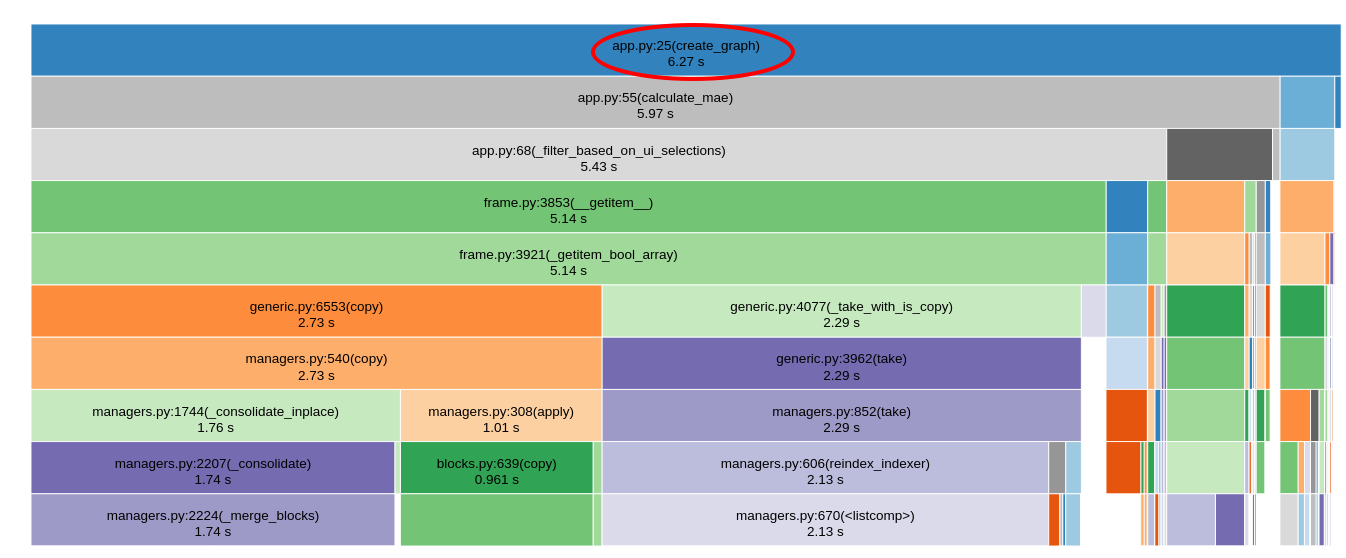
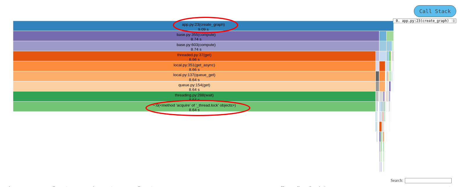
@pn.io.profile("profile", engine="snakeviz")
def create_graph(
    file: str,
    minute_of_day: tuple[float, float],
    identifiers: list[int],
):

    client = get_client()
    minute_of_day = tuple(map(round, minute_of_day))

    future = client.submit(get_data_for_graph, file, minute_of_day, identifiers)
    mae_a, mae_b = future.result()
    mae_a = mae_a.compute()
    mae_b = mae_b.compute()

    common_opts = dict(legend="top")
    graph_scatter_pipeline = mae_b.hvplot.scatter(
        label="B", **common_opts
    ) * mae_a.hvplot.scatter(label="A", **common_opts)

    return graph_scatter_pipeline

it will throw an exception:

ModuleNotFoundError: No module named 'bokeh_app_30c15ce7b3b248ec93ee1ae6185c16f7'

The above exception was the direct cause of the following exception:

Traceback (most recent call last):

... [omitted]

RuntimeError: Error during deserialization of the task graph. This frequently
occurs if the Scheduler and Client have different environments.
For more information, see
https://docs.dask.org/en/stable/deployment-considerations.html#consistent-software-environments

Full traceback

2024-01-24 16:52:28,756 Error running application handler <bokeh.application.handlers.script.ScriptHandler object at 0x7f6e6048b070>: Error during deserialization of the task graph. This frequently
occurs if the Scheduler and Client have different environments.
For more information, see
https://docs.dask.org/en/stable/deployment-considerations.html#consistent-software-environments

File 'client.py', line 330, in _result:
raise exc.with_traceback(tb) Traceback (most recent call last):
  File "/home/niko/code/myproj/.venvs/venv/lib/python3.10/site-packages/distributed/scheduler.py", line 4671, in update_graph
    graph = deserialize(graph_header, graph_frames).data
  File "/home/niko/code/myproj/.venvs/venv/lib/python3.10/site-packages/distributed/protocol/serialize.py", line 439, in deserialize
    return loads(header, frames)
  File "/home/niko/code/myproj/.venvs/venv/lib/python3.10/site-packages/distributed/protocol/serialize.py", line 101, in pickle_loads
    return pickle.loads(x, buffers=buffers)
  File "/home/niko/code/myproj/.venvs/venv/lib/python3.10/site-packages/distributed/protocol/pickle.py", line 96, in loads
    return pickle.loads(x)
ModuleNotFoundError: No module named 'bokeh_app_30c15ce7b3b248ec93ee1ae6185c16f7'

The above exception was the direct cause of the following exception:

Traceback (most recent call last):
  File "/home/niko/code/myproj/.venvs/venv/lib/python3.10/site-packages/bokeh/application/handlers/code_runner.py", line 229, in run
    exec(self._code, module.__dict__)
  File "/home/niko/code/myproj/app.py", line 126, in <module>
    main_graph = pn.panel(imain_graph)
  File "/home/niko/code/myproj/.venvs/venv/lib/python3.10/site-packages/panel/pane/base.py", line 87, in panel
    pane = PaneBase.get_pane_type(obj, **kwargs)(obj, **kwargs)
  File "/home/niko/code/myproj/.venvs/venv/lib/python3.10/site-packages/panel/param.py", line 799, in __init__
    self._replace_pane()
  File "/home/niko/code/myproj/.venvs/venv/lib/python3.10/site-packages/panel/param.py", line 865, in _replace_pane
    new_object = self.eval(self.object)
  File "/home/niko/code/myproj/.venvs/venv/lib/python3.10/site-packages/panel/param.py", line 824, in eval
    return eval_function_with_deps(function)
  File "/home/niko/code/myproj/.venvs/venv/lib/python3.10/site-packages/param/parameterized.py", line 162, in eval_function_with_deps
    return function(*args, **kwargs)
  File "/home/niko/code/myproj/.venvs/venv/lib/python3.10/site-packages/param/depends.py", line 41, in _depends
    return func(*args, **kw)
  File "/home/niko/code/myproj/.venvs/venv/lib/python3.10/site-packages/param/reactive.py", line 431, in wrapped
    return eval_fn()(*combined_args, **combined_kwargs)
  File "/home/niko/code/myproj/.venvs/venv/lib/python3.10/site-packages/panel/io/profile.py", line 251, in wrapped
    return func(*args, **kwargs)
  File "/home/niko/code/myproj/app.py", line 63, in create_graph
    mae_a, mae_b = future.result()
  File "/home/niko/code/myproj/.venvs/venv/lib/python3.10/site-packages/distributed/client.py", line 322, in result
    return self.client.sync(self._result, callback_timeout=timeout)
  File "/home/niko/code/myproj/.venvs/venv/lib/python3.10/site-packages/distributed/client.py", line 330, in _result
    raise exc.with_traceback(tb)
RuntimeError: Error during deserialization of the task graph. This frequently
occurs if the Scheduler and Client have different environments.
For more information, see
https://docs.dask.org/en/stable/deployment-considerations.html#consistent-software-environments

Full MWE code

# Run with:
# python -m panel app.py --autoreload --show --args  [data_file]
from __future__ import annotations

import sys


import dask.dataframe as dd
from dask.distributed import Client
import pandas as pd
import hvplot.pandas  # noqa
import hvplot.dask  # noqa
import panel as pn


def get_data(file) -> dd.DataFrame:
    df = dd.read_parquet(file)
    for i in range(15):
        df[f"extra_col{i}"] = df["val_A"] + i
    return df


@pn.cache  # share the client across all users and sessions
def get_client():
    return Client("tcp://127.0.0.1:8786")


def get_data_for_graph(
    file: str,
    minute_of_day: tuple[float, float],
    identifiers: list[int],
):

    df = get_data(file)

    mae_a = calculate_mae(
        df=df,
        label="A",
        minute_of_day=minute_of_day,
        identifiers=identifiers,
    )
    mae_b = calculate_mae(
        df=df,
        label="B",
        minute_of_day=minute_of_day,
        identifiers=identifiers,
    )
    return mae_a, mae_b


@pn.io.profile("profile", engine="snakeviz")
def create_graph(
    file: str,
    minute_of_day: tuple[float, float],
    identifiers: list[int],
):

    client = get_client()
    minute_of_day = tuple(map(round, minute_of_day))

    future = client.submit(get_data_for_graph, file, minute_of_day, identifiers)
    mae_a, mae_b = future.result()
    mae_a = mae_a.compute()
    mae_b = mae_b.compute()

    common_opts = dict(legend="top")
    graph_scatter_pipeline = mae_b.hvplot.scatter(
        label="B", **common_opts
    ) * mae_a.hvplot.scatter(label="A", **common_opts)

    return graph_scatter_pipeline


def calculate_mae(
    df: dd.DataFrame,
    minute_of_day: tuple[int, int],
    identifiers: list[int],
    label: str,
) -> dd.Series:
    df_filtered = _filter_based_on_ui_selections(
        df, minute_of_day=minute_of_day, identifiers=identifiers
    )
    mae = do_calculate_mae(df_filtered, label=label)
    return mae


def _filter_based_on_ui_selections(
    df: dd.DataFrame,
    minute_of_day: tuple[int, int],
    identifiers: list[int],
) -> dd.DataFrame:

    df_filtered = df[df["minute_of_day"].between(*minute_of_day)]
    return df_filtered[df_filtered["identifier"].isin(identifiers)]


def do_calculate_mae(
    df: dd.DataFrame,
    label: str,
) -> dd.Series:

    col_err = f"err_{label}"
    df[col_err] = abs(df[f"val_{label}"] - df["val_C"])
    mae = df.groupby("minute_of_day")[col_err].agg("mean")

    return mae


pn.param.ParamMethod.loading_indicator = True
pn.extension(sizing_mode="stretch_width", throttled=True)


dfraw = get_data(sys.argv[1])
unique_ids = list(dfraw["identifier"].unique())

minute_of_day = pn.widgets.RangeSlider(
    name="Minute of day", start=0, end=1440, value=(0, 1440), step=10
)
identifiers = pn.widgets.MultiChoice(
    name="Identifiers", options=unique_ids, value=unique_ids
)
imain_graph = pn.bind(
    create_graph, file=sys.argv[1], minute_of_day=minute_of_day, identifiers=identifiers
)
main_graph = pn.panel(imain_graph)

minute_of_day.servable(area="sidebar")
identifiers.servable(area="sidebar")
main_graph.servable(title="Data graph")

What is happening here? Why dask works without Panel, but not with it? What is this unpickling of bokeh_app_30c15ce7b3b248ec93ee1ae6185c16f7 ?

Edit: Solution

I found this comment from the bokeh discourse:

Bokeh dynamically creates module new module objects every time a user session is initiated, and the app code is run inside that new module for isolation. If you are saving/reading between different sessions.

I also figured out the reason. The reason is that panel uses bokeh, and bokeh creates dynamically a new module for each browser session. When calling client.submit, or more generally, when sending tasks for Dask like this:

future = client.submit(somefunction, *args)

the somefunction is also sent to the Cluster as a pickled function. The pickling process includes having to know the module and the function name. The summary of this is that all functions that are processed in Dask must be defined outside a bokeh app module (because of that random naming the modules get). I know that Scaling with Dask — Panel v1.3.7 says

the Client and Cluster must able to import the same versions of all tasks and python package dependencies

but I think it would be better for Dask+Panel beginners that it would also explicitly say that you cannot process any functions with Dask which are defined in your app.py (main Bokeh / Panel module).

fohrloop · January 29, 2024, 12:22pm

Hi all, just giving an update. @ahuang11 suggested to look at the dask dashboard. It shows real difference when using obj.hvplot.scatter() when obj is either a dask object or a pandas object (series or dataframe).

If running obj.hvplot.scatter() and obj is a dask object, the you’ll see something like this in the dask scheduler dashboard:

All of those darker blue boxes read the parquet file. Now if I call the obj.compute().hvplot.scatter(), effectively using hvplot with pandas, and running my own scheduler with single worker, I will see something like this:

I don’t know a reason for this but it seems that the hvplot.scatter does something else than just calls obj.compute. For some reason the workload is split into much smaller chunks with dask+hvplot than when just computing everything with dask.

(the data shown in the above figures is not the MWE but from another similar app)

ahuang11 · January 29, 2024, 3:12pm

I think the chunk size might be the issue; I’d recommend checking out Dask Best Practices — Dask documentation

philippjfr · January 30, 2024, 9:21am

Thanks for all your investigation here, could you try something for me and use: obj.persist().hvplot.scatter()

fohrloop · January 30, 2024, 10:50am

@ahuang11 I also would guess it’s something related to the chunk size but I don’t understand why the chunk size is different if using daskobj.hvplot.scatter(). The reference gallery entry for hvplot Scatter does not mention chunk size. Not sure where it should be defined…

@philippjfr I’ll try that. First I update the MWE do it is possible to use it with the dask dashboard. Here is updated code:

Updated MWE

This time it is in form for installable package:

📁 panel-mwe/
├─📁 myproj/
│ ├─📄 app.py
│ ├─📄 task.py
│ └─📄 __init__.py   # empty file
└─📄 pyproject.toml

pyproject.toml

[project]
name = "myproj"
description = "myproj"
version = "0.1.0"
dependencies = [
    "dask[distributed]",
    "panel",
    "hvplot", 
    "pyarrow", 
]

[build-system]
build-backend = "flit_core.buildapi"
requires = ["flit_core >=3.2,<4"]

myproj/app.py

from __future__ import annotations


import dask.dataframe as dd
from dask.distributed import Client
import hvplot.dask  # noqa
import hvplot.pandas # noqa
import panel as pn

import sys

from myproj.task import get_data, get_mae


@pn.cache
def get_dask_client() -> Client:
    client = Client("tcp://127.0.0.1:8786")
    return client


def create_graph(
    file: str,
    minute_of_day: tuple[float, float],
    identifiers: list[int],
):
    client = get_dask_client()
    minute_of_day = tuple(map(round, minute_of_day))

    mae_a = client.submit(
        get_mae,
        file=file,
        minute_of_day=minute_of_day,
        identifiers=identifiers,
        label="A",
    ).result()
    mae_b = client.submit(
        get_mae,
        file=file,
        minute_of_day=minute_of_day,
        identifiers=identifiers,
        label="B",
    ).result()

    common_opts = dict(legend="top")
    graph_scatter_pipeline = mae_b.hvplot.scatter(
        label="B", **common_opts
    ) * mae_a.hvplot.scatter(label="A", **common_opts)

    return graph_scatter_pipeline


pn.param.ParamMethod.loading_indicator = True
pn.extension(sizing_mode="stretch_width", throttled=True)


minute_of_day = pn.widgets.RangeSlider(
    name="Minute of day", start=0, end=1440, value=(0, 1440), step=10
)
unique_ids = [21, 79]
identifiers = pn.widgets.MultiChoice(
    name="Identifiers", options=unique_ids, value=unique_ids
)
imain_graph = pn.bind(
    create_graph, file=sys.argv[1], minute_of_day=minute_of_day, identifiers=identifiers
)
main_graph = pn.panel(imain_graph)

minute_of_day.servable(area="sidebar")
identifiers.servable(area="sidebar")
main_graph.servable(title="Data graph")

myproj/task.py

from __future__ import annotations

import dask.dataframe as dd
import panel as pn


@pn.cache
def get_data(file) -> dd.DataFrame:
    df = dd.read_parquet(file)
    for i in range(15):
        df[f"extra_col{i}"] = df["val_A"] + i
    return df


def get_mae(
    file: str,
    minute_of_day: tuple[int, int],
    identifiers: list[int],
    label: str,
) -> dd.Series:
    df = get_data(file)
    df_filtered = _filter_based_on_ui_selections(
        df, minute_of_day=minute_of_day, identifiers=identifiers
    )
    mae = do_calculate_mae(df_filtered, label=label)
    return mae


def _filter_based_on_ui_selections(
    df: dd.DataFrame,
    minute_of_day: tuple[int, int],
    identifiers: list[int],
) -> dd.DataFrame:
    df_filtered = df[df["minute_of_day"].between(*minute_of_day)]
    return df_filtered[df_filtered["identifier"].isin(identifiers)]


def do_calculate_mae(
    df: dd.DataFrame,
    label: str,
) -> dd.Series:
    col_err = f"err_{label}"
    df[col_err] = abs(df[f"val_{label}"] - df["val_C"])
    mae = df.groupby("minute_of_day")[col_err].agg("mean")

    return mae

Commands

Setting up: Create a virtual environment, activate it, and install the myproj. Run in the project root (same folder with pyproject.toml)

python -m venv venv
source venv/bin/activate
python -m pip install -e .

Starting:

First, start the dask scheduler and a worker. These need to be ran in separate terminal windows, and both need to have the virtual environment activated (+any changes to the app require restarting both of these)

dask scheduler --host=tcp://127.0.0.1 --port=8786
dask worker tcp://127.0.0.1:878

then start the panel app:

python -m panel serve myproj/app.py --show --admin --args ~/Downloads/testdata.parquet

The data file link is in the first post.

MWE results

I’m using more powerful computer than in the OP. Here only one worker on dask.

Using `daskobj.hvplot.scatter`:

code

    # mae_a and mae_b are dask series
    graph_scatter_pipeline = mae_b.hvplot.scatter(
        label="B", **common_opts
    ) * mae_a.hvplot.scatter(label="A", **common_opts)

results

Initial load 19 seconds, filtering ~14 seconds

one task (initial load, filtering) looks like this

Using `pandasobj.hvplot.scatter`:

Add a .compute() to convert dask serie to pandas serie:

code changes

    mae_a = (
        client.submit(
            get_mae,
            file=file,
            minute_of_day=minute_of_day,
            identifiers=identifiers,
            label="A",
        )
        .result()
        .compute() #here
    )
    mae_b = (
        client.submit(
            get_mae,
            file=file,
            minute_of_day=minute_of_day,
            identifiers=identifiers,
            label="B",
        )
        .result()
        .compute() #here
    )

    common_opts = dict(legend="top")
    graph_scatter_pipeline = mae_b.hvplot.scatter(
        label="B", **common_opts
    ) * mae_a.hvplot.scatter(label="A", **common_opts)

results

About 10 seconds for page load, and 2-3 seconds for filtering

The dask Task Stream looks much better. Each task (initial load, filtering) produces something like this:

The `daskobj.persist().hvplot.scatter`

code changes

    mae_a = client.submit(
        get_mae,
        file=file,
        minute_of_day=minute_of_day,
        identifiers=identifiers,
        label="A",
    ).result()
    mae_b = client.submit(
        get_mae,
        file=file,
        minute_of_day=minute_of_day,
        identifiers=identifiers,
        label="B",
    ).result()

    common_opts = dict(legend="top")
    graph_scatter_pipeline = mae_b.persist().hvplot.scatter( # persists here
        label="B", **common_opts
    ) * mae_a.persist().hvplot.scatter(label="A", **common_opts)

results

Speed from the panel admin:

8 sec initial load
About 2 seconds to filter afterwards

Initial page load and filtering produce something like this in the dask dashboard:

Reference: using only pandas

results

4 sec page load, 1-2 sec for filtering

Summary of results

pandas only: 4 sec initial load, 1-2 sec filtering
dask + dask.hvpot: 19 sec initial load, 14 sec filtering
dask.compute() + pandas.hvplot: 10 sec initial load, 2-3 sec filtering
dask + dask.persist().hvplot: 8 sec initial load, 2 sec filtering

jerry.vinokurov · February 4, 2024, 1:53am

@fohrloop Interesting investigation, thanks for doing all that. One thought that occurs to me is that one of the issues you might be running into is that everything is happening in your main namespace; it should be possible to serialize and deserialize a function that is imported from a module without running into this problem. In that case, Dask should be able to import that same function from the same module as long as the environments are consistent.

fohrloop · February 5, 2024, 8:33pm

@jerry.vinokurov if you’re referring to the fact that all the code was in a single module in the original post, that is correct. I learned here the hard way that Dask pickles your functions and unpickles them in the workers, which has it’s own problems when using it in a panel (or bokeh) app. Only this last MWE has a separate task.py for Dask. But yeah, you’re absolutely right in all that. And when dealing with editable installs, the scheduler and worker needs to be restarted every time the modules have changes (this bite me few times).

I actually ended up ditch Dask from the equation as I found out that in my use case (10Gb-100Gb data in memory) Dask is not the best option. I first got 5 minutes page loads/response times with Dask, then got that down to 1:30 minutes with some optimizations. The distributed processing with the IPC is not the most efficient way for non-big data. Nowadays the coolest new things seem to be DuckDB and Polars. I got today 40-50 seconds loading times with Polars on the first try; about twice faster than the somewhat optimized Dask version, and I’m about to try to optimize it a bit. DuckDB is on the todo list. And these both support out-of-core computing (data larger than RAM). I wish I can get it to the 5-10 seconds range with these

ahuang11 · February 7, 2024, 4:47am

Also, just to throw this out there there’s Ray too

fohrloop · April 11, 2024, 10:47am

I ended up using DuckDB. Some benchmarks with my 24Gb parquet file (71Gb in memory. All of that will not fit into memory at once. Tested on my laptop):

Dask: 5:00min initially, 1:30min with optimizations
Polars: 40 seconds out of the box. 11 seconds with some fine tuning.
DuckDB: 0.5-2 seconds out of the box (used same optimized table structure as with Polars)

I liked the Polars API perhaps a bit more than writing SQL for DuckDB, but decided to go with DuckDB as it was so fast out of the box.

ahuang11 · April 11, 2024, 5:28pm

Yes I like duckdb too!

Why Panel is 10x slower with Dask than with Pandas?

Code for MWE app:

Running the code

Test data

Edit: Additional Benchmarks

Question

Profiling (app using Dask)

The profiling code

Profiling results

Profiling with pandas

Profiling results

Summary

Question

Using .compute() before creating hvplots

Results

Just Dask, no Panel

Dask within Panel App

Edit: Solution

Updated MWE

Commands

MWE results

Using daskobj.hvplot.scatter:

Using pandasobj.hvplot.scatter:

The daskobj.persist().hvplot.scatter

Reference: using only pandas

Summary of results

Using `daskobj.hvplot.scatter`:

Using `pandasobj.hvplot.scatter`:

The `daskobj.persist().hvplot.scatter`